Walk-Through: Build a Compartmental Model
You can build simple compartmental models of neurons using the Network module in Neurosim. Such models can form part of a circuit that interacts with other neurons. As an example, we will build a compartmental model consisting of a cell body with a branching dendrite receiving synaptic inputs, and an axon for output. The soma and axon will carry HH-type spikes, but the dendrites will be passive. We will then connect it to some single-compartment integrate-and-fire neurons, to show the interoperability possibilities.
But first, here are some activities to familiarize yourself with the general commands and procedures used in constructing compartmental models.
Warm-Up
If you have not already done the Network Walk-Through Warm-Up, I suggest you do that before proceeding.
- Load and Start the file compart warm-up start.
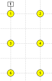
There are 6 stand-alone non-spiking neurons in the Setup view (panel a in the figure below). N1 receives an excitatory stimulus pulse which depolarizes it, but since there are no connections between the neurons and each neuron is independent, none of the others shows any response.
Linking and Unlinking Compartments
- Clear the Results view (you cannot reconfigure compartments in a model while results are visible).
- Drag a box around all the 6 neurons to select them.
- Their borders are drawn with a thick line, indicating selection.
- Select the Neuron: Compartmental model: Link selected neurons menu command.
- De-select the 6 compartments by clicking the mouse anywhere in the Setup view away from a compartment/neuron.
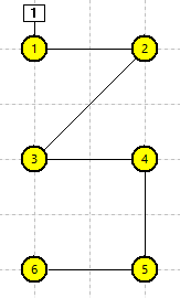
This links all the selected neurons into a linear chain in ID order, such that each neuron is now a compartment within a single 6-compartment neuron. Note that the "neurons" are now connected by straight lines, indicating intracellular continuity between connected compartments (panel b in the figure below). The zig-zag in the connection line is simply due to the layout order of the 6 compartments in the view - you could re-arrange the compartments into a straight line by dragging them if you wished.
So we now have a compartmental model. How does it behave?
A Detour on Integration Time Step and Stability
- Click Start.
Failure! When the simulation run reaches the time of the start of the stimulus, a message pops up saying that the calculation has generated an impossibleIntegration failure can sometimes just result in chaotic output, without generating an impossible number. This is usually obvious in the Results view, when the traces oscillate wildly between extreme values. number, and the run terminates. There are two related underlying problems. First, with this model the default integration time step (0.5 ms) is far too long for the numerical integration method (exponential Euler) used in Neurosim.
- Clear the Results view.
- Select the Options: Integration menu command to open the Integration dialog.
- Set the Integration time step to 0.001 ms.
- Click OK to dismiss the dialog.
- Click Start.
The simulation now runs to completion, but it is very slow for such a simple model.
This takes us to the second problem. The 6 compartments are each 50 µm in diameter and only 50 µm in length (the diameter of the original neurons - see Implementation details). This means that there is a very low axial resistance between compartments, and hence even a tiny voltage difference between compartments generates a relatively large axial current flow, causing a very steep rate of change in voltage. That is why the integration time step has to be so short. The issue is apparent when you look at the Results view. There is very little attenuation of the depolarization between N1 at the top of the view, and N6 at the bottom (about 0.06 mV drop). So the entire model is almost isopotential. We could generate almost equally accurate results with a considerably larger step size (and hence a faster simulation run) by making the compartments longer relative to their diameter. We will see how to do that later.
Now we return to editing the model.
- Clear the Results view.
- Drag a box around N3 and N4 (the middle row) to select them.
- Select the Neuron: Compartmental model: Unlink selected neurons menu command.
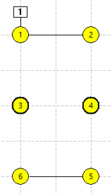
N3 and N4 are now once again stand-alone neurons, while N1 + N2 and N5 + N6 form two independent 2-compartment neurons (panel c in the figure below). N3 and N4 should still be selected.
- Select the Neuron: Compartmental model: Link selected neurons menu command.
- De-select the compartments.
Now we have three 2-compartment neurons!
- Select the Neuron: Compartmental model: Link 2 neurons menu command.
- Drag the mouse from N2 to N3 to link them as compartments.
- Repeat, but this time drag from N2 to N5.
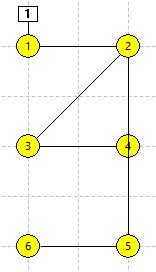
The connecting line goes through N4, but does not connect to it (panel d in the figure below).
The Setup view is now quite confusing, but the anatomy can be clarified by rearranging the layout of the compartments. Drag each compartment until it matches the layout in panel e in the figure below. It should now be obvious that we have a 6-comparment model of a branching structure, such as a part of a dendritic arbor.
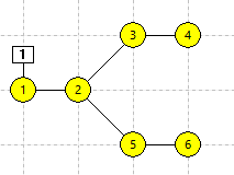
Note: now that the model has a branching structure, we would have to reduce the integration time step even further to run it successfully! The simulation would probably then be too slow to be useful.
Anatomy
At the moment the model has 6 nominally spherical compartments. A spherical compartment is suitable for a cell body, but not for a dendrite or axon - these should be cylindrical.
- Double-click N1 to open its Neuron properties dialog, and move the dialog so that it does not obscure the Setup view layout.
- Select the Shape: Cylinder option.
- Set the Diameter to 15 µm and the Length to 200 µm.
Note in the Setup view that N1 now displays as a horizontal rectangle, representing the cylinder.
- Return to the Properties dialog and check the permission box beside each of the 3 options that you adjusted (Cylinder, Diameter and Length).
- Enter 2-6 into the Extended Apply list box near the bottom of the dialog.
- Click the Apply button.
All 6 compartments now show as horizontal rectangles. However, they are a bit small (and soon some will be smaller still), so it would be nice to enlarge the view.
- Select the Options: Configure view menu command to open the Configure view dialog.
- Change the Default neuron radius to 20.
Note that the units here are relative display units (pixels), not actual anatomical units. - Click OK to close the dialog.
- Change the Default neuron radius to 20.
The rectangles are now considerably larger in the Setup view. This is purely cosmetic - there is no change in the underlying model, just in the size at which structures are drawn in the view.
- Drag the rectangles so that they do not overlap.
At this point the model could look like panel a in the figure below.
- Return to the Properties dialog and set the Source to 5.
- Select the Vertical option for the Orientation.
- Click Apply.
- Repeat for Source 6.
Compartments 5 and 6 are now drawn as vertical rectangles. They appear to be "dangling" from the compartmental connection drawn across their upper ends (panel b in the figure belowN5 and N6 were dragged slightly to activate snap-to-grid.). However, this is just a result of the way they are drawn - connections between adjacent compartments are always drawn between the ends of the respective rectangles that are geometrically closest in the Setup view. It is up to the model constructor to arrange the Setup view layout so that it gives an intuitive representation of the anatomy. (However, note that in terms of the calculation driving the simulation itself, the connection is from centre-to-centre of the linked compartments and the layout does not matter; see Implementation details.)
- Drag N6 so that it is below N5.
The layout now makes more sense (panel c in the layout below).
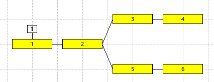
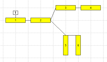
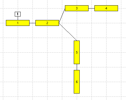
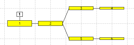
- Return to the horizontal layout as in panel a above (I won't give step-by-step instructions here - it's a challenge !!).
At the moment the compartments in our dendritic tree model are all the same size (15 x 200 µm). However, in real neurons, more distal dendrites tend to taper as branching progresses, so let's introduce that into the model.
- Select Source 2 in the Properties dialog.
- Set the Diameter to 8 µm.
- Click Apply.
- Repeat, to set N3 and N5 to 6 µm diameter, and N4 and N6 to 3 µm diameter.
- Click OK in the Properties dialog to close it.
- Drag a compartment to activate the snap-to-grid facility to align the compartments neatly.
At this point the Setup view should look like panel d in the figure above.
A note on Setup view scaling: In compartmental models in Neurosim, dimensions in the Setup view scale with the square root of dimensions in the real (virtual) neuron. Thus a compartment with 20 µm diameter is actually 4x wider than one with 5 µm diameter, but will only appear 2x wider in the Setup view. This means that if one compartment is anatomically larger than another in the real neuron, it will always appear larger in the Setup view too, but not in direct proportion. This is a design decision taken in order to keep small objects visible and clickable in the same Setup view as large objects.
Also note that in the current version of Neurosim, cylindrical compartments can only be orientated vertically or horizontally, not obliquely.
The model is now anatomically more realistic than the previous version with spherical compartments. How does it run?
- Set the integration time step to 0.05 ms as described previously.
- Click Start.
The simulation now runs more quickly (a result of the larger integration step size), and is still stable. You can experiment with even larger step sizes, to see what happens ...
- Adjust the top axis scales to -30 mV (top) and -65 mV (bottom) to make the data more visible.
- Select the View: Same scale menu command.
- Since no axis is selected, this sets all voltage scales to those of the top axis.
- If a sub-set of scales were selected, only those would be affected.
For your convenience, compart warm-up finish is a pre-built version of the warm-up model at this stage.
Intracellular Resistivity (Ri)
With data showing in the Results view:
- Double-click a compartment to open its properties.
- Change the Ri (intracellular resistivity) from 100 to 1000 Ωcm.
- The new resistivity value (which is probably unrealistically high, but which emphasizes the effect) is a global parameter that applies to all compartments within the model.
- Click Start.
- Use the Highlight sweep facility to switch between the Results with 100 and 1000 resistivity values.
The increased internal resistance increases the voltage response in N1 (the compartment receiving the stimulus) because less of the injected current spreads internally into the adjacent compartment. In N2, the response is virtually unchanged because the reduced inflow of current from N1 is more-or-less balanced by a reduced outflow to N3 and N5. However, for the distal compartments N3-6 the voltage response is reduced because they receive less overall current. Effectively, the length constant of the dendritic tree has been reduced by the increased internal resistance, just as it would be for a linear uniform cable.
Compartment Size? Integration Step Size?
The simplifying assumption underlying all compartmental models is that individual compartments are isopotential - i.e. there is no voltage difference between different regions within a compartment. Obviously, this is never actually true, but the shorter the compartment, the closer it gets to being true. However, as we have seen, short compartments require small integration time steps for the calculation to remain stable, and, of course, they also require more compartments to represent a given anatomy, which means more calculations and slower simulations. So the aim is to make both the compartments and the integration time steps as large as possible without sacrificing too much accuracy. The question is, how large is that?
Sadly, the answer is largely heuristic. For integration step size, it is easy to reduce the step size and run the simulation again. If there is no significantI don't mean statistically significant, I just mean within an acceptable error range. difference in the output, then the original step size was suitable. If there is a significant difference, then repeatedly reduce the size until the difference becomes insignificant!
For compartment size, a commonly used rule-of-thumb is that they should be no longer than 10% of the space constant of an infinitely-long length of passive dendrite with the same the properties as the compartment. Thus if we assume a space constant of 5 mm (a fairly typicalBut be aware that the nominal space constant applies to DC signals, and that the effective space constant is shorter for high-frequency signals due to the low-pass filter characteristics due to membrane capacitance. value), then compartments should be shorter than 500 µm. Again, if you are concerned about the accuracy of the model, then the best that I can suggest is to reduce the compartmental size (thus increasing the number of compartments), and see if the output changes.
Finally, bear in mind that most models will contain at least some numerical parameters that are "guesstimates" rather than accurate values derived from experimental data. Small changes in these parameters may affect the model output at least as much as micro-fine-tuning the compartment sizes to increase apparent accuracy.
A Compartmental Model with Active and Passive Components
The second part of the walk-through is to build a model containing both active (i.e. spiking) and passive components. The spikes will be simple HH spikes, based on the squid giant axon.
- If you want to keep the dendritic model that you just built, save it now.
Soma
First we need to get a neuron with HH spikes into a Network model. The easiest way is to copy one from the Advanced HH model.
- Select the Model: Advanced HH menu command to launch the Advanced HH model.
- The default neuron in this model carries HH spikes
- Set the diameter to 20 µm.
- This just keeps everything a bit smaller than the default.
- Select the Neuron: Copy menu command.
You have now placed a single spherical neuron with 20 µm diameter and HH spike channels onto the clipboardIn this case the clipboard format is bespoke for Neurosim - the neuron can only be pasted into the Network or Advanced HH model in an instance of Neurosim itself.. This will form the soma in our new compartmental model.
- Select the Model: Network menu command to switch to the Network module, which will start with the default 2-neuron circuit.
- Right-click N1 and select Paste neuron from the context menu.
- This "converts" N1 into the neuron that we placed on the clipboard.
- If you had right-clicked away from any neuron, you would have pasted a new neuron into the model, but we may as well use the existing neuron.
- Right-click N2 and select Delete neuron from the context menu.
- Right click the square stimulus box 2 and select Delete stimulus from the context menu.
We now have a neuron with HH channels in a Network model. This will become the soma in our compartmental model, but it is probably a good idea to test it to make sure everything works as expected.
- Select ms as the Time unit in the Experimental Control panel to the left of the Setup view.
- This is simply because it will easier to work with milliseconds rather than seconds as our time units.
- Select stimulus 1 in the Stimulus frame of the Experimental Control panel (normally docked to the left of the Setup view).
- Change the stimulus Duration from 100 to 1 ms.
- Change the Delay to 2 ms.
- In the Results view, set the right-hand timebase scale to 20 ms.
- Set the top scale of axis 1 to 40 mV.
- Click Start.
You should see a single spike-like waveform in the N1 trace of the Results. This is encouraging, but the waveform looks very "chunky".
- Clear the Results view.
- Select the Options: Integration menu command to open the Integration dialog.
- Set the Integration time step to 0.01 ms and click OK to dismiss the dialog.
- Click Start.
The spike waveform now looks more respectable! But the neuron in the Setup view is a bit too small for comfort.
- Select the Options: Configure view menu command to activate the Configure View dialog.
- Set the Default neuron radius to 15.
- Set the Grid spacing to 32.
- Click OK to dismiss the dialog
- Drag N1 towards the top-centre of the Setup view.
- Set the Default neuron radius to 15.
These changes are cosmetic - they affect the layout in the Setup view, but do not affect the model itself. The changes will make things easier later.
- Double-click the neuron to open its Properties dialog.
Note that Na and K channels appear within the Voltage-dependent channels list.- Change the Description text to "soma". This will be accurate later!
- Click OK to dismiss the dialog.
If you want to check your progress, the parameter file compart 1 contains the model so far.
Now we will add an axon to the soma.
Axon
- Select the Neuron: Multi-add: Placeable menu command.
- Click the Setup view six times in a vertical row beneath the soma, clicking on every other grid node, to place 6 new neurons.
- Right-click the mouse anywhere (or press ESC) to finish adding new neurons.
At this stage we have 7 separate neurons, each carrying HH channelsWhen you add new neurons in this way, they inherit the properties of the most recent neuron previously added to the circuit.. However, we want these to be compartments within a single neuron.
- Drag the mouse to form a box around all 7 neurons to select them.
- Select the Neuron: Compartmental model: Link selected neurons menu command.
A connecting line is now drawn between the 7 yellow circles, indicating that they are now compartments within a single neuron. However, at the moment we have a neuron with 7 somata and no axon!
- Double-click N2 to open its Neuron Properties dialog.
Note that the Compartment option box at the top-centre of the dialog is now checkedIt is checked automatically because the program detects that this "neuron" is actually linked as a compartment to other "neurons" (compartments)., which makes compartment-relevant options visible within the dialog. As it happens, the default values are all appropriate for the soma compartment (N1), but not for the putative axon (N2-7).
- Change the Description to "axon"
- Select the Vertical option for Orientation.
- Select the Cylinder option for Shape
- Set the Diameter to 5 µm.
- Set the Length to 200 µm.
As you make these changes, note how the N2 display changes in the Setup view. - Leave the Ri at 100 Ωcm
- Check the box beside the 5 parameters that you changed (Description, Orientation, Geometry, Diameter and Length) to give permission to copy these to other compartments.
- Enter 3-7 into the Extended Apply list at the bottom of the dialog.
- Click Apply.
You should now see the axon as a vertical line of cylinders. - Click OK to dismiss the Properties dialog.
- If necessary, drag the cylinders so that they line up neatly under the soma.
Because Snap to grid is selected by default, (see Options: Configure view) all the compartments should align on grid nodes.
Now let's check whether our axon conducts.
- Click Traces in the Result view to open the Trace and Axis Setup dialog again.
- Enter 7 into the Neuron box for axis 2.
- Its Show box should already be checked from the original configuration.
- Click OK to close the dialog.
- Click Start.
The stimulus, which previously generated a spike in the soma when it was isolated, is now subthreshold. This is because the extra load of the axon acts as a current sink on the soma.
- Select Stimulus 1 (either by clicking the box in the Setup view, or by clicking 1 in the stimulus list in the Experimental control panel).
- Increase the Amplitude to 0.8 nA.
- Click Start.
The soma should now generate a spike, which propagates along the axon.
At the stage the Setup and Results view should look like this:

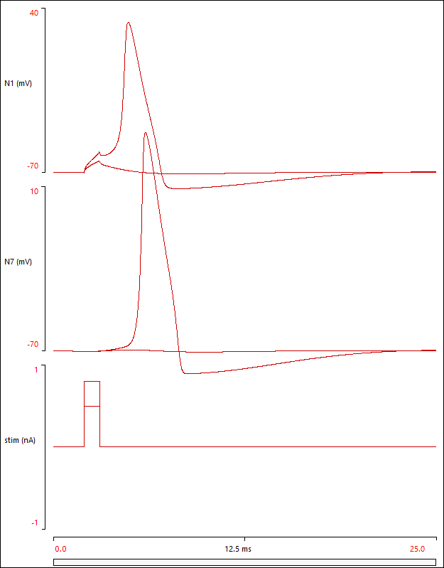
The parameter file compart 2 contains the model so far.
Dendrites
- Clear the Results view.
- Control-drag N7 (the terminal compartment of the axon) and drop it above the soma compartment.
- Shift the stimulus marker to the side, and maybe move the whole soma-axon structure down to make room.
This duplicates the axonal N7 compartment as N8, but N8 is not linked into the compartmental structure, so it is not (yet) part of the neuron.
- Double-click the new N8 compartment to open its Properties dialog.
- Click the Del all button in the Voltage-dependent channels frame near the bottom.
This removes both the HH voltage-dependent channels (Na and K), thus making the compartment passive. - Change the Description to "dendrite".
- Change the Leak equilibrium potential to -70 mV.
This is so that the resting potential of the passive dendrite compartments matches that of the active HHThe voltage-dependent channels make a small contribution to the resting potential, so to get the same resting potential, the leakage channel equilibrium potential is different in active compartments from that in passive compartments. compartments. - Click OK to close the dialog.
- Click the Del all button in the Voltage-dependent channels frame near the bottom.
- Select the Neuron: Compartmental model: Link 2 neurons menu command.
The cursor changes to a purple up-arrow. - Drag from N8 to N1 (or vice versa) to link N8 into the neuron model as a passive dendritic compartment.
- Duplicate N8 by control click-and-drag to produce three new compartments to the right of N8, and three new compartments to the left of N8. Drop the new compartments on every other grid node, as before.
You should now have 6 new isolated cylindrical compartments, N9 - N14.
- Drag around N9, N10 and N11 to select them.
- Select the Neuron: Compartmental model: Link selected neurons menu command to link the N9-N11 as compartments.
- Repeat for N12-N14.
At the moment, the dendrites are all aligned vertically, and they appear to be linked at their top ends. In fact, compartments are always functionally linked centre-to-centre in terms of the calculation, but the links are drawn between the closest ends in the Setup view display.
- Double-click N9 to open its Properties dialog.
- Select the Horizontal option for Orientation.
Note how N9 changes from vertical to horizontal orientation. - Check the box beside the option.
- Enter 10-14 in the Extended Apply list.
- Click Apply.
All the new dendritic compartments should now be horizontally aligned. - Click OK to close the Properties dialog.
- Select the Horizontal option for Orientation.
- Link N8 to N9 using the Neuron: Compartmental model: Link 2 neurons menu command as before.
- Repeat to link N8 to N12
- If necessary, drag the compartments to make a tidy display.
The dendrites should form a branching T-shape above the soma. - Click the Traces button in the Results view to open the Trace and Axis Setup dialog.
- Check the Show boxes for axes 4 and 5.
- Enter 11 and 14 into the Neuron(s) boxes for axes 4 and 5 respectively.
- Edit the Axis label for axes 4 and 5 appropriately.
- Click OK.
We will need an even bigger stimulus than before, because the new passive dendrites increase the load on the soma.
- Increase the stimulus 1 amplitude to 2 nA.
- Change the stimulus (3rd) trace scales to 0 - 2 nA.
- Click Start.
At this point the Setup and Results display should look something like this (your Setup arrangement may differ from mine, but the Results should be the same):
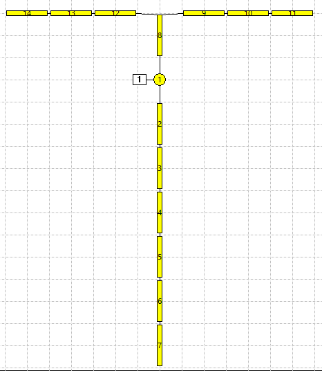
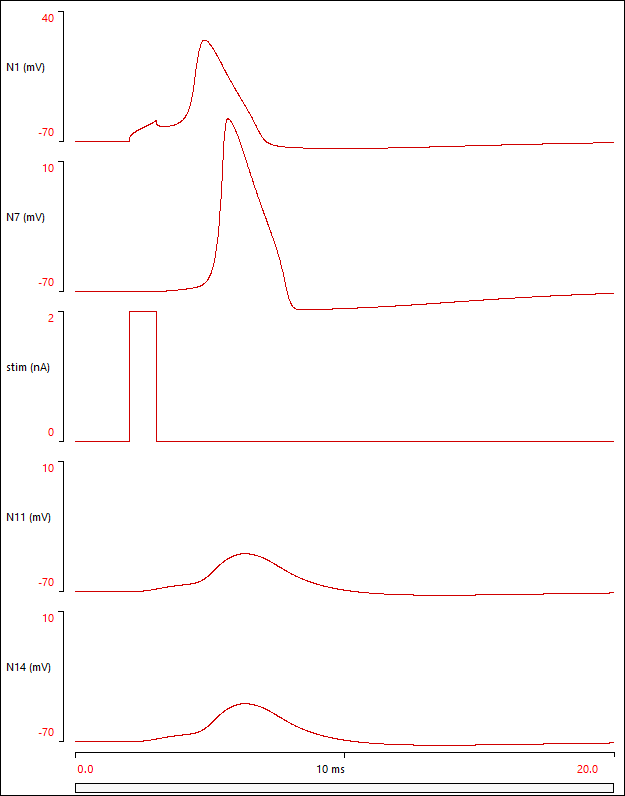
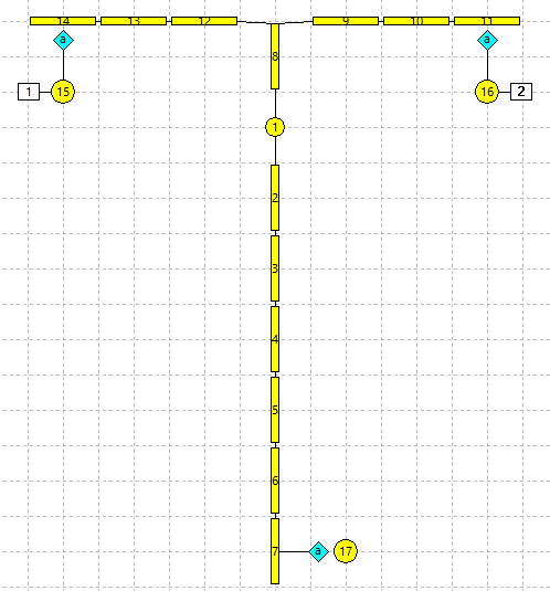
Note that a spike is initiated in the soma (N1) and spreads by active conduction along the axon to its terminal (N7), but also back-propagates into the dendritic arbor through passive conduction, to produce a depolarizing potential at the distal dendrite tips (N11, N14).
The parameter file compart 3 contains the model so far.
Build Into a Circuit
We have now completed the compartmental model. It is very simple, but hopefully this walk-through demonstrates most of what is needed for building more complex models, if desired.
How can this model be incorporated into a circuit with other neurons?
- Select the Neuron: Add menu command, and click below the tip of the left-hand dendrite (N14 in the Setup in the figure above).
The new neuron (N15) inherits the dendritic properties of the last compartment added, but we want it to be a standard single-compartment integrate-and-fire neuron.
- Double-click N15 to open its Properties dialog.
- Select Spherical Geometry.
- Set the Diameter to 30 µm.
- Check the Use integrate-and-fire spikes box in the Integrate-and-Fire frame.
- Set the AHP conductance to 4 mS/cm2.
- Uncheck the Compartment options box to hide compartment-related options.
This last change is not strictly necessary, but it may prevent confusion later. - Change the Description to "single-compartment neuron".
- Click OK to close the dialog.
- Control click-and-drag N15 to duplicate it just under the right-hand dendrite tip (N11 in the figure above).
- Control click-and-drag N15 to duplicate it beside the axon terminal (N7).
We now have 3 stand-alone single-compartment integrate-and-fire neurons, N15, N16 and N17.
- Clear the Results view (if it is not already clear).
- Click the Results Traces button to open the Trace and Axis Setup dialog (again).
- Check the Show boxes for axes 6, 7 and 8.
- Enter 15, 16 and 17 into the Neuron(s) boxes for these axes, and edit the Axis labels appropriately.
- Change the stimulus box contents of axis 3 to 15 16.
There is no stimulus applied to these neurons yet, but there will be soon. - Click OK to close the dialog.
- In the Setup Experimental Control panel, set the Target neuron for stimulus 1 to 15.
The stimulus box in the Setup view moves from N1 (the soma) to N15. - Move the stimulus box to the left-hand side of N15.
- Reduce the Amplitude of stimulus 1 to 1 nA.
- Select the 0 (new) stimulus in the stimulus list.
Note that the stimulus parameters are copied from the existing stimulus 1. - Set the Target neuron to 16.
This sets up a new stimulus 2 applied to N16. - Move the stimulus box to the right-hand side of N16.
- Set the Delay for stimulus 2 to 3.5 ms to delay it slightly with respect to stimulus 1.
- Click Start to see where we are.
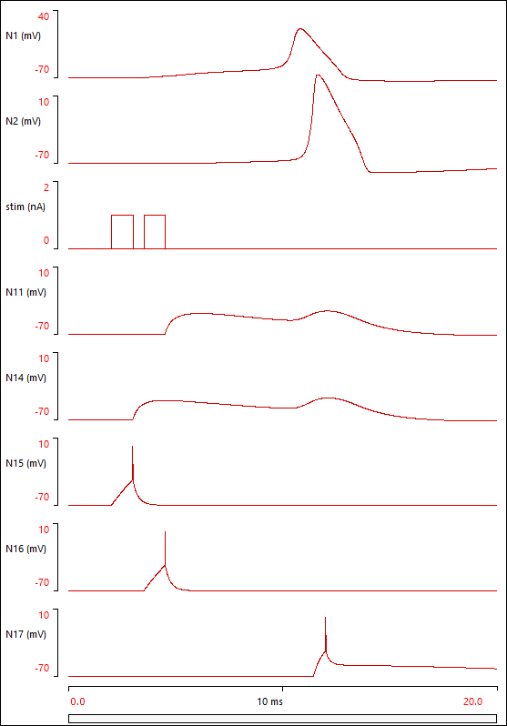
You should see slightly offset spikes in N15 and N16. These are integrate-and-fire neurons, so the spikes are actually just digital events with minimal duration - their appearance is basically cosmetic. However, these spikes will activate synapses, once we set them up.
- Clear the Results view.
- Select the Connexions: Multi-add menu command.
- Click-and-drag the mouse from N15 (the new stand-alone neuron) to N14 (the nearby dendrite tip).
- Click OK to accept the default settings in the Synaptic Connexion dialog that pops up.
This sets up excitatory (nicotinic ACh) synaptic input from N15 to the distal tip of one of the dendrites of the compartmental neuron.
- Repeat for N16 to N11.
This sets up input to the distal tip of the other dendrite. - Repeat for N7 to N17.
This sets up synaptic output from the axon terminal to N17. - Right-click (or press ESC) to terminate the multi-add process.
N7 is a spiking compartment, where the spike is modelled with HH kinetics (it is not an integrate-and-fire type). By default, synaptic output from N7 is triggered when the membrane potential crosses a threshold value in the positive direction.
- Double-click N7 to open its Properties dialog.
- Note that Synapse trigger level is set at 0 mV. An HH-type spike will cross this level on its rising phase, so this is satisfactory.
- Click OK to close the dialog.
Note: if we wanted a more sophisticated synaptic response where the EPSP was dependent on the shape of the spike (width etc.) , we could use a suitably tuned "non-spiking" synapse, where transmitter release depends on the spike properties, rather than being an all-or-none event. But for this walk-through, we will stick with the simple mechanism.
- Click Start.
There is a barely-perceptible depolarization in the dendrite tip compartments (N11 and N14), and the compartmental neuron certainly does not spike. Clearly the synaptic input does not generate enough current to have a significant effect. We need a stronger synapse!
- Clear the Results view.
- Select the Synapses: Spiking chemical menu command to open the Spiking Chemical Synapse Types dialog.
- Increase the Synaptic conductance for type a (the default nicotinic ACh type) from 0.1 to 1.5 mS/cm2.
- Click OK to close the dialog.
- Click Start.
The two pre-synaptic neurons (N15, N16) spike, and produce EPSPs in the distal dendrite tips of the compartmental neuron (N14, N11). The depolarization spreads by passive conduction to the soma (N1), and there is sufficient temporal and spatial summation to depolarize the soma above threshold. The soma consequently spikes. The spike propagates to the end of the axon (N7), where it triggers synaptic output onto N17, which also spikes in response to the EPSP it receives from the axon output.
The spike in the soma also propagates by passive conduction out into the dendrites, where it produces a late depolarizing "backwash" on the falling phase of the EPSPs.
At this point the Setup and Results display should look something like this:
The parameter file compart 4 contains the finished model.
The importance of the post-synaptic summation can be demonstrated by removing one of the pre-synaptic inputs.
- Select stimulus 2 in the Experimental Control panel.
- Click the down spin arrow to reduce the Amplitude of the stimulus to 0.9 nA.
- Click Start.
The stimulus to N16 is now subthreshold and the neuron does not spike. Consequently there is no EPSP in one of the dendrites and no summation. The remaining EPSP generated by N15 does not take the compartmental neuron above threshold, and consequently there is no spike in its axon, and no output to N17.
