Contents
Template-Based Event Detection
Template-Based Detection
Store/Retrieve templates
Error metric
Average template
Subtract from trace
Increase frequency
Adaptive templates
Optimal scale/offset
Multi-Trace Templates
Template-Based Waveform (Spike) Detection
One common use of events is to mark the time of occurrence of waveform fragments with a particular shape, such as spikes generated by a single axon within an extracellular recording showing the combined activity of several axons. One way of doing this is through template-based event creation.
- Load the file cpr. You should see about half of the entire record displayed on the screen, and it should look like this:

The data show an extracellular recording from the ventral nerve cord of a crayfish. A light was switched on shortly after the start of the recording, and most but not all of the spikes are from the caudal photoreceptor (CPR). These are the spikes we want to analyse.
- Select the Sound: Play menu command to get a sense of the activity pattern.
- Select the Windows: New Window command.
We now have two identical views of the same data file, cpr.dtvw-dat:1 and cpr. dtvw-dat:2 appearing in the title bars of the display windows. - Select Windows: Tile main view so that you can see both views at once.
- In window 2 set the start time of the second window to 1600 by editing the left-hand horizontal axis value, and set the end time of the display to 1625. (Note that you MUST press the tab key after you enter a new value into an edit box, to make the program aware of your entry.)
You should see a single spike more-or-less centered in the screen. Normally you would locate this or a similar spike using the navigation controls within the program, but for the tutorial it is important that you pick the same spike that I did, so that the numbers work out the same.
Generate a template
- Select the Cursor: Place at time menu command to place a vertical cursor at 1611 ms.
- Repeat to place a second cursor at 1612 ms.
The two cursors should bracket the displayed spike. Again, normally you would place these by eye, using the mouse to drag them to the correct positions.
- Select the Event edit: Template recognition menu command to activate the Template event recognition dialog.
Note that this is a modeless dialog, so you can carry out other actions without having to dismiss it (and if it gets in the way of the display, you can minimize it).
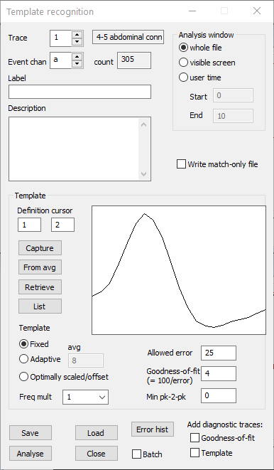
- Click the Capture button in the Template recognition dialog. The waveform appears in the window in the middle of the dialog: this is the template that will be used in the search.
The dialog should now look like this:
- You can now get rid of the cursors in the expanded main view (2) using the Cursors: Del all vert menu command.
Detect template matches
You are now ready to search the recording for waveforms that match this captured template. The closeness of match required is set by the Allowed errorThere is also a Goodness-of-fit parameter, but this is simply the reciprocal of the allowed error multiplied by 100 parameter, which has a default value of 25 (the error metric is explained below). Any matches that are found will be marked as events in channel a.
There are two other facilities that can aid in waveform detection if viewed during the process, so we will activate these now.
- Select the Event analyse: Event triggered scope view menu command to display the Scope view. There are no events yet, so at the moment the display is empty.
- Select the Event analyse: 2-D scatter graph menu command to show the Scatter graph with its default Frequency vs time display. This too will be empty at this stage.
You are now ready to search for matches to the template.
- Click the Analyse button at the bottom left of the Template recognition dialog.
After a brief pause, the Template recognition dialog informs you that 305 waveforms have been found that match the template, and the scatter graph and the scope view now become populated. However, there are three problems:
- In the Scope view, the initial part of the waveforms are quite similar but there are clearly two categories distinguishable in the later part of the display.
- The Frequency vs time scatter graph shows a clear pattern that matches with the overall visual appearance of the recording in the main view, but there are many high-frequency outliers that are unlikely to come from the same neuron since they would require an unusually short refractory period.
- In the long-timebase main view (1) events mark many extracellular spikes, but this includes the low-frequency spikes at the start of the recording, before the light stimulus was applied.
It therefore seems likely that non-cpr spikes have been included in the analysis.
- In the Template recognition dialog, reduce the Allowed error to 12. This means that waveforms will have to be more similar to the template than previously to be regarded as a match.
- Click Analyse.
Now only 239 spikes are recognized as template matches. The spikes visible in the Scope view now look identical within the limits of noise, and the high-frequency outliers have disappeared from the Scatter graph. Furthermore, in the long timebase main view (1) the pre-stimulus spikes are no longer marked by events. This is much better!
A comparison of the Scope view and scattergraphs is shown below:
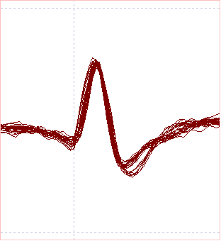
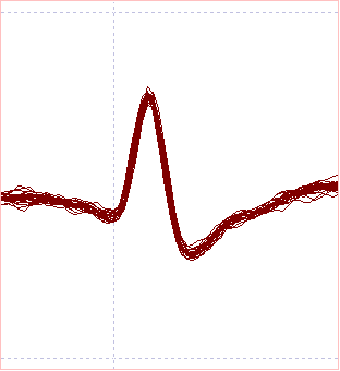

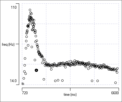
The Scope view and Scatter graph data suggest that with the lower allowed error, the spikes generated by the crayfish CPR have been identified with reasonable accuracy.
The other spike
Deciding on the original spike to use as a template was in this case a matter of luck (with a bit of judgement). What happens if you chose the wrong spike?
- In the zoomed-in window, set the start time to 100 ms.
A single spike should be visible on the left. This is one of the pre-stimulus spikes.- Set vertical cursors at 106 and 107 ms.
- In the Template recognition dialog
- Change the Event channel to b.
- Reset the Allowed error to 25.
- Capture a new template.
- Analyse the data.
The Scope view and Scatter graph look very much like they did with the previous template.
- Reduce the Allowed error to 12 and re-Analyse.
Now the other spike has been identified. This neuron spikes at low frequency throughout the recording and is unaffected by the light stimulus.
If we had chosen the "wrong" spike for our initial template, we would have had two choices: try again after choosing another spike for the template and hope for better luck, or stay with the larger allowed error to detect both spikes, and use the spike sorting technique described here, or the Spike-Sorter Wizard described here, to separate them out.
- Delete event channel b.
- Save the cpr file with the new name cpr event using the File: Save as menu command. The new file should automatically load, and should be identical to the cpr file, including the new event channel.
For your convenience, this file is also available for download: cpr event. - Close the original cpr file without saving it. If you use the File: Close menu command both views will close, if you use the X at the top-right of the window frame, you will have to close each view separately.
Storing and Retrieving templates
When Dataview performs a waveform recognition analysis, it stores a copy of the template with the event channel, and thus we can retrieve the template from the event channel itself. This would allow us to re-analyse the data using the same template, should that be necessary.
- In the new file that you previously saved (cpr event), open the Template event recognition dialog box from the Event edit: Template recognition menu command.
Initially the Retrieve button in the dialog is disabled because the default event channel is set to an empty channel (in this case b) to reduce the risk of inadvertently overwriting events acquired previously. The events are stored in channel a, and so this is where the template is also stored.
- Change the channel selection to a in the dialog
- Click the Retrieve button and the template should appear in the display window. Note that the Allowed error is also retrieved.
Of course, templates are only available in event channels that were initially established by template recognition.
Template error metric
The error metric used in Dataview is simply the sum of the absolute deviation of the recorded waveform from the template, normalized such that an error of 100 is that generated by a waveform identical to the template, but shifted on the Y axis by half the peak-to-peak value within the template. This is calculated on a point-by-point basis throughoutOr rather, throughout the region of the recording selected for analysis. The user can opt to only analyse part of a long recording. the recording. If the error drops below the allowed value, the search continues until the error once again exceeds the allowed value, and the template-length section of data with the lowest error in the preceding within-tolerance region generates an event.
- If you changed the expanded timebase before saving the cpr file, set the start time to 1600 and the end time to 1625 ms, to centre the template spike again.
- Note that the event (id 58) is labelled "template", and is tagged (drawn with a thicker outline).
- Select the Event edit: Event channel properties menu command to activate the Event channel properties dialog.
- Note that channel a is selected by default.
- Select Template error from the drop-down Numeric display per event list. (This option only occurs in the list if the event channel was derived by template recognition.)
- Click OK.
In the main view note that the template event now shows a value of 0. This is because the waveform is an exact match to the template - not surprising, of course, since this waveform is the template.
- Click the right page toolbar button (
 ).
).
Two new spikes come into view with event values of 7.67 and 9.65. Both have been recognized as template matches within the allowed error of 12 - the values show how close the match is.
Error value
Determining an appropriate value for the allowed error is often done heuristicallyMeaning by trial-and-error, but that phrase introduces too many errors into the sentence, as well as not sounding very professional., using the Scope view and Scatter graph as aids. However, you can also examine the error distribution itself, which can help the decision.
- With the template retrieved into the Template Recognition dialog as described above, click Analyse. This should produce identical results to previously, but it also makes information about the error distribution available.
- Click the Error hist button near the bottom of the dialog to display the Template error histogram.
The histogram shows the point-by-point error between the data and template throughout the analysis region. There is a single point in the zero-value bin at the far left of the histogram caused by the exact match (zero error) between the template and the data spike used to create the template. There is then a collection of bins, with a trough occurring at the (draggabble) red cursor. The X-axis value is the error, and the existence of this trough is the reason that the Allowed error value of 12 was chosen. (You can hover the mouse over the histogram to display the X-axis value in the Error at mouse box.)
- Change the X-axis maximum scale to 100, and check the Auto scl Y box. You may want to increase the width of the histogram by dragging on a side edge.
You should now see a huge set of bins centred around an error of about 60. These are caused by the error between the template and the interspike baseline noise where there are no spikes. This generates the vast majority of the data points in the histogram at this scale.
- Un-check the Auto scl Y box and set the Y-axis maximum to 100.
The histogram should now look like this:
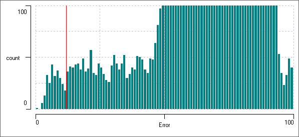
You can see the error signal distribution remains relatively flat up to about 46, before it takes off towards the huge baseline error. There is a trough at the location of the red cursor (error 12), and, with the eye of faith, you can also see a trough in the histogram at about error 28. Drag the red cursor to this position.
- Close the Template error histogram dialog.
Note that the Allowed error in the main Template recognition dialog has now been set to the cursor value (about 28).
- In the Template recognition dialog, reset the Allowed error to 12.
- Change the Event channel to b to avoid overwriting your original analysis.
- Select the Event analyse: Event triggered scope view menu command to open the Scope view again.
- Set the event channel to b (which is empty at the moment, so nothing displays).
- Set the count (in the Sweeps to draw group) to -1. This means that all event waveforms will display, rather than just the default of the first 25.
- Click Analyse in the Template recognition dialog. (The Allowed error should be at its original value of 12; the first trough in the error histogram you just looked at.)
The Scope view should show a very "clean" spike display. - Increase the Allowed error to 28 (the second nominal trough in the error histogram) and click Analyse.
A second spike which is similar but not identical to the first becomes visible in the Scope view. - [Perhaps click the 'Heat' plot button in the Scope view. See here for details.]
- Increase the Allowed error to 42 (just before "take off" in the error histogram) and click Analyse.
There are now some small signals in the Scope view which are clearly poor matches to the template, but none-the-less have a spike-like shape. - Increase the Allowed error to 60 (well into the noise in the error histogram) and click Analyse.
There are now a large number of almost flat signals in the Scope view which are basically just membrane noise.
Saving the error as a trace
Another facility that helps in getting a feel for this type of analysis is to display the error signal and/or template as a trace.
- In the Template recognition dialog, return the Allowed error to 12.
Note that the Goodness of fit value is now 8.33+. - Check the goodness-of-fit box in the Add diagnostic traces group at the bottom-right of the dialog.
- Click the Analyse button. A File save dialog box appears, in which you should enter a name for the new data file that will contain the error signal trace. After a brief interval the new file should load automatically.
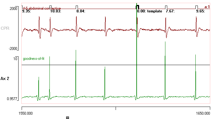
The error signal is displayed on the lower trace of the new file as a Goodness-of-fit signal (equivalent to 100 divided by the error), so positive shifts in this trace indicate improvements in the fit.
- In the new file, set the start time to 1550 and the end time to 1650.
You should now see several spikes, some of which are recognized as matches to the template, while others are not. - Select the Cursors: Place at voltage menu command to open the Place horizontal cursor dialog.
- Enter 8.3333 into the Place at value edit box.
- Enter 2 into the relative to trace edit box.
- Click OK to place the cursor.
The horizontal cursor should now be positioned at the goodness-of-fit threshold. The spike waveform is only recognized as a match to the template when the lower trace crosses the cursor.
Averaging templates
- Reload the file that you saved with your original template match (allowed error 12), Retrieve the waveform from event channel a, and re-Analyse the file.
You should once again generate 239 events.
Note that there is a button From avg just below the Capture button. The template was originally defined by capturing a section of trace from the raw data, and obviously in most cases this waveform will be contaminated with noise. The template recognition algorithm will try to find matches to the noise as well as the underlying signal, which results in sub-optimal identification of genuine matches.
- Click the From avg button. This replaces the original template with a template formed from the average of all the event waveforms currently recognised within the channel. This obviously tends to “centre” the template waveform and reduces the risk of false positive or negative recognition.
- Change the Event channel to b.
- Click the Analyse button.
This time 243 events are recognized, which are slightly more that we had previously.
Subtract Average Spike from Trace
Once a spike has been identified it can be useful to remove it from a trace to see what is left.
- Load the new file that you previously saved (cpr event).
Expand the timebase by setting it to 100 ms/div, and set the Start time to 500 ms (this is just so you can see the spikes better).
- Save the file with a new name (e.g. cpr subtract spikes).
- Copy event channel a into event channel b using the Event edit: Logical operation: EQUALS (copy) menu command.
- Activate the Event-triggered scope view from the Event analyse menu.
- With the trigger channel set to b, click the Disp = Ev(1) button. This sets the display to exactly match the event duration.
You now see precisely what was matched to the template. The key features of the spike are encompassed, but you do not see its entire waveform.
- Set the Sweep dur to 4.5 and the Start to -0.8. You should now see just about the entire spike waveform.
- Check the Avg (average) box. This waveform is what we want to subtract from the raw data, at precisely the times of the matched spikes.
- Click the Ev = Disp button. Events in channel b now match this expanded waveform.
We are now ready to do the actual subtraction. You can dismiss the Scope view, or leave it running if you wish.
- Select the Transform: Set data values in events menu command to activate the appropriate transform dialog.
- Set the event channel to b, and select the Subtract within-event average of source option. The other default choices are OK.
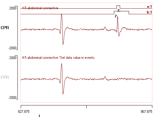
- Click the Preview button. The upper black trace shows the original signal, while the lower red trace shows the signal after subtracting the average cpr spike waveform for each identified spike.
The original recording has a slight baseline offset due to to electronic drift in the amplifier. This is included in the average, and so when subtracting the average, the offset is removed over the time of the spike. This is not what we want, since it produces a discontinuity in the transformed trace.
- Uncheck the Compensate baseline offset box, and observe the discontinuity appearing in the Preview at the time of each removed spike. Re-check the box again to remove it.
The compensation works by taking the average of the first and last points within the template as a measure of the offset. This is then added back to the signal after removing the average waveform. This is one reason why it is important to encompass the entire spike waveform in events in the controlling channel.
- Finally, click the OK button. Select a name for the new file, and have a look at it after it loads. It should look something like this:

On-the-fly frequency increase
- Load the file cpr lf4.
This is exactly the same as file cpr that was used previously, except that the sample frequency has been reduced by a factor of 4 from 20 kHz to 5 kHz by decimation. This still meets the Nyquist criterion, but it means that a simple “join the dots” display of the waveforms produces considerable distortion.
- Generate a template in the Template recognition dialog as described previously, except set the vertical cursors at 1611 and 1612.1 ms (i.e. with the second cursor slightly later due to the need to capture at least 5 data points).
The template is very "angular" due to the relatively low sample frequency (red trace in a, below). - With the Allowed error set at 12, click Analyse.
Note that only 54 spikes are recognized. - Now select 8 from the Freq mult drop-down list.
The apparent template sample rate is increased by a factor of 8 (i.e. to 40 kHz), and the template waveform now looks like a smooth spike. The original reduced-frequency waveform is shown in red in the dialog, while the up-sampled waveform is shown in black (below, a).
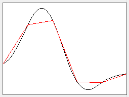

- Click Analyse and note that now 243 spikes are recognized as matches to the template, which is quite an improvement on 54!
The analysis takes considerably longer because the raw data are being up-sampled in real time as the search for a template match progresses. We could achieve a similar effect by using the Transform: Increase frequency facility to up-sample the entire file, but this would increase the overall file size by a factor of 8, whereas the on-the-fly increase leaves the original data unchanged.
- Activate the Scope view and note that the matched waveforms now look very disparate because they are displayed at the original (reduced) sample rate (above, b).
If you want to retrieve the waveform of the up-sampled template, click List. If you want to get the average up-sampled waveform of the recognized spikes, click From avg before you click List. You can also write a new file containing just the up-sampled matched waveforms by checking the Write match-only file box before you click Analyse.
Adaptive template matching
It sometimes happens that a waveform undergoes a systematic change during the course of a recording session. This may be due to things like deterioration in the recording quality (e.g. suction electrodes losing their suck) or some systematic change in neural properties (spike broadening etc). In these cases it is useful to have a template that can update itself as the waveform changes.
- Load the file fade out.
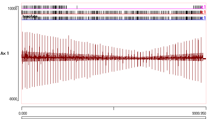
This shows an extracellular recording on which an event analysis was performed to detect a particular spike (the first spike in the record provided the template). The resulting events are stored in event channel b.
- Click the Show all toolbar button (
 ).
).
After the event detection was performed, a filter was applied to this file first to gradually reduce the amplitude of the signal, and then to restore it again.
We will perform an identical event analysis on the filtered data.
- Open the Template event recognition dialog.
- Set the Event channel to b. Note that there are 206 events in the channel.
- Click the Retrieve button. This places the template that was used to acquire channel b into memory.
- Now change the event channel to a and click Analyse.
The Event count box shows that now only 65 spikes are detected, some at the beginning and some at the end of the trace, but no spikes are detected in the middle where the amplitude has dropped.
- Now change the Event channel to c.
- Change the Template type option from Fixed to Adaptive.
- Click Analyse, and watch the template waveform displayed in the capture window. This shrinks and then grows again. Note there are now again 200+ events detected.
- Expand the main view time-base until you can clearly see the individual events, then go to the start of the record.
- Hold down the control key, and then repeatedly press the e key. You will hop from event to event through the record. If you simply keep the e key pressed, the keyboard auto-repeat facility will scroll you through each recognized event in turn.
You should see that event channel c (constructed using the adaptive template) closely matches event channel b (constructed before filtering the data), but that event channel a misses all the events in the middle of the record where they have shrunk in amplitude.
The adaptive template works by replacing the original template with a running average of the waveforms of recognised events. The number of events constituting the average is set in the Adaptive avg edit box (default 8), and as each new event is recognised, the earliest event in the average drops out to be replaced by the most recent. If you select an average of 1, then the template is successively replaced by each identified event, so that each found event constitutes the template for the next event search.
- Close the file fade out.
Optimally scaled template matching
The fixed template mode of recognition is used when you want to find events in the waveform that closely match the selected template in all respects (shape, size and dc-offset). However, there are occasions when you are looking for events that are the same shape as the template, but which may vary from it in both amplitude and mean potential. A classic example is the detection of miniature synaptic potentials, which all have a similar shape of waveform, but which vary considerably in amplitude.
In this situation the Optimally scaled/offset option is appropriate. This utilises an ingenious algorithm described by Clements & Bekkers (1997). The basic idea is that you start with a “pure” template with normalized amplitude and no noise. Clements and Bekkers constructed their templates using a mathematical equation to describe the waveform, but in DataView the template is captured from the data. The template is then passed through the data record on a successive point-by-point basis, and at each point it is optimally scaled and offset (the equations that do this are the clever bit of the algorithm) to produce the best possible match to the segment data at that point. The standard error between this optimally scaled and offset template and the data is then calculated. The ratio between the scale factor and the standard error is taken as a goodness-of-fit criterion. Since the original template is normalised to an amplitude of 1, the scale factor measures the real amplitude of the matched template in the signal, and thus the acceptance criterion is closely related to the signal-to-noise ratio of the selected waveform in the data. The goodness-of-fit criterion is thus affected by two factors, the size of the waveform in the data, and the closeness with which its waveform matches the optimally scaled template. A goodness-of-fit criterion value of about 4 usually provides a good balance between missing genuine event matches, and capturing false ones. (All of this information comes from the cited paper.)
- Load the file quantal. Note the initial waveform marked as a template.
- Click the Show all toolbar button (
 ).
).
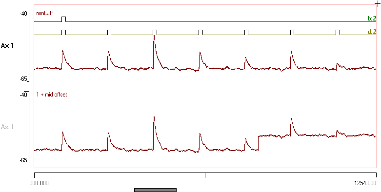
Trace 1 is simulated data (constructed using Neurosim) showing quantal variation in miniature EJPs in response to constant-frequency 20 Hz stimulation. Trace 2 is exactly the same as trace 1, except a DC offset has been added to the mid region for testing purposes.
The first potential near the beginning of the record was used as a template, and using standard Template recognition with an Allowed error of 12 the program detected just 4 events in trace 1 that matched that template EJP. These are stored in channel a. In trace 2 only 2 events were detected (stored in channel b), because the offset in the mid region prevented a match to the other EJPs. None of the larger or smaller EJPs were detected, which is as it should be.
A fragment of the recording before and after analysis with the optimally scaled/offset facility is shown below:
To help the next stage of analysis:
- Select the Event analyse: Event triggered scope view menu command to display the Scope view.
- Set the count to -1 to show all the sweeps.
- Select the Event analyse: 2-D scatter graph menu command to show the graph with its default Frequency vs time display.
- Set the event channel to c in both dialogs, which will now become empty because there are not yet any events in channel c.
Now we can try the optimally scaled/offset facility.
- Call up the Template recognition dialog.
- Retrieve the template from channel a.
- Select the Optimally scaled/offset option.
- Set the event channel to c.
- Set the trace to 1 (i.e. the trace without the mid offset)
- Click Analyse.
Now 61 waveforms are detected. The Scope view shows many EJPs, but also one almost flat sweeps. The Scatter graph shows a steady frequency pattern at 20 Hz, but with a pair of high outliers.
- Expand the main view timebase by setting the scale to 50 ms/div.
- In the Scope view, click on the almost flat sweep. This will centre the outlier event in the main view.
The problem is that there is a small deviation in the baseline noise that happens to match a massively reduced version of the EJP waveform.
- In the Template dialog, set the Minimum pk-2-pk amplitude to 1 (located below the Capture display on the right). This means that waveforms must have at least this peak-to-peak amplitude to be recognized as a match.
- Click Analyse again.
There are now 60 waveforms recognized as a match, and the Scope view shows that these all look like EJPs. Furthermore the Scattergraph shows a uniform frequency distribution, which is as it should be because the EJPs were elicited by stimulation at fixed frequency.
What about the trace with the offset?
- Set the Recognition event channel to d and the trace to 2.
- Click Analyse.
Again, 60 events are detected. If you switch the event channels in the Scope view and Scattergraph between c and d there is no change in the display. The optimal offset part of the algorithm successfully discounts the offset introduced into trace 2.
Multi-Trace Template Match
It is sometimes useful to detect repeating patterns of activity that span several different traces, and the Event edit: Multi-Trace Template option provides this facility.
- Load the file crawling.
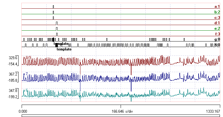
This shows activity in the motorneuron pool of the 3 most posterior abdominal segments in a fly larvae, as monitored by fluorescence of a calcium indicator dye (data kindly provided by Dr Stefan Pulver, University of St Andrews). The waves of activity relate to abdominal contractions as the animal is crawling, and visual inspection shows at least two patterns. There are relatively sharp-peaked waves that progress from anterior to posterior (up the screen) indicating backwards crawling, and broader and flatter waves that are relatively synchronous, which indicate forwards crawling. The single events in event channels a, b and c mark waves in one sequence of a backwards crawl, while events in channels d, e and f mark a sequence of a forwards crawl. The events were inserted manually after visual inspection, to mark what was judged to be a “typical” episode of each type. Channels a and d have trace 1 set as their parent, b and e have trace 2, and c and f have trace 3.

Before starting the analysis it is helpful to activate the Scope view so that the recognitio parameters can be "tuned" while viewing the outcome.
- Activate the Event-Triggered Scope View (Event analyse menu).
- Set the Trigger channel to g. This is the channel that will eventually hold the results.
- Set the Count to -1 (show all sweeps).
- Set the Sweep duration to 10000, and the Start (re trig) to -3000. The crawling waves are slow, and so the timescale must be long.
Of course, at this time there are no events in channel g and so the Scope view is blank.
- Activate the Multi-Trace Template Recognition dialog using the menu command above.
- Enter a b c as the Source channels (spaces are optional, abc will also work)
- Click Capture.
Note the waveform that displays in the dialog: this is the section of waveform in trace 1 encompassed by the single event in channel a, and it acts as one of the templates. You can view the other templates by selecting them from the drop-down Primary template list. The displayed template acts as the primary template, the non-displayed templates are the secondary templates. The difference will be explained in a moment.
- Click the Analyse button.
The program searches trace 1 for all sequences that match the Primary template (assuming this is still defined by channel a). It uses the same search error criteria as described previously. In this case it finds 48 matches, as indicated by the Primary count value in the Recognition dialog. It then goes on to search for matches to the secondary templates, as follows. For each primary match, it searches trace 2 for a match to the template defined by channel b and trace 3 for a match to the template defined by channel c, but these matches have to occur in the same time relation to the primary match as the channel b and c events have to the channel a event. If does not find matches at the appropriate times, then the primary match itself is deleted. The result is that the events in the Destination channel g reflect episodes in the recording where the waveform pattern expressed in traces 1, 2 and 3 match, within the specified error, those underlying the template events. With the current settings there are 10 such episodes, of which several are visible on screen, with the match to the template episode highlighted.
The specifications as set require an exact match in timing, and this is quite restrictive.
- Change the Search slack parameter from 0 to 500 (a value chose by experiment).
- Click Analyse again.
Now the program searches within a time window that extends 0.5 s on either side of the “expected” time defined by the templates, and two more episode matches are discovered. However, there are many apparent episodes of backwards crawl which have not yet been detected, including several visible in the display.
- Check the Optimally scaled/offset box.
- Click Analyse again.
Now the program scales and offsets each section of data to achieve the closest fit to the template, before checking the match in terms of the Allowed error (this is described in more detail earlier). This means that waveforms which are the same shape as the template, but differ in amplitude, can be detected as matches. Now we find 68 matches to the primary template, and 30 matches to the full template pattern.
You can now interactively adjust the Allowed error and/or Search slack (in the template dialog) to try to optimize detection, while observing the detected pattern in the Scope View. With an Allowed error of 35, 36 episodes of the backwards crawl pattern are detected (below a).
Increasing the allowance much beyond this starts to bring in patterns that are not good matches to the template.
Now we will try to find the other pattern. In the Template dialog box
- Enter d e f as the Source channels.
- Click Capture.
- Set the Destination channel to h.
- Set the Scope view event channel to h as well.
- Click Analyse and note that 42 episodes are detected.
- In the Scope View set the Trigger channel to h and note the different pattern.
- Increase the Allowed error to 50.
- Click Analyse again and note that now 56 episodes are detected, but all show more-or-less the same pattern (below b)
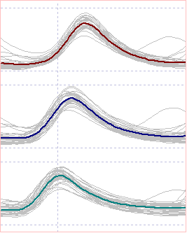
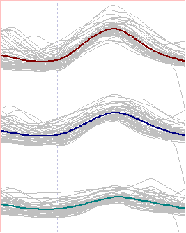
In the main view display click the Show all toolbar button (below, channels a–f hidden). The recording is from an experiment in which a drug was applied between the two obvious “glitch” markers in the traces. You can see that prior to drug application (the left of the screen) most of the episodes are matched by events in channel g, indicating that they are backwards crawls, but after drug application there are many more events in channel h, indicating forwards crawling.
