The Nyquist frequency and data acquisition
There is an important general point to be made about sampling frequency. This may be common knowledge amongst experts, but many people (all right, I, at any rate) have been confused by it.
It is commonly stated, and true, that if an AD converter runs at a sample rate that is twice the highest frequency contained within the analogue signal (the Nyquist frequency) then the digitized signal will contain all the information that was present in the analogue signal. However, this does not mean that a straightforward display of the digitized data by “joining the dots” will look like the original signal. In order to reconstruct the original signal from digitized data sampled at the Nyquist criterion it is necessary to output the data as a series of impulses, and to pass these impulses through a low-pass filter that has a cut-off frequency equal to the Nyquist frequency. If this is done then the output from this filter will indeed be a replica of the original input signal. However, this is not easily achieved in practice, and is not part of the processing of most digital data display systems, including DataView. If you want the digital data display to look something like the original analogue signal using a simple join-the-dots algorithm, you will almost certainly have to sample at well above twice the Nyquist frequency. But under any circumstances, you absolutely must ensure that the sample frequency of the AD converter is more than twice the frequency of any signal contained in the analogue data, or the dreaded aliasing will occur (an example of which is given below).
Decimation and Interpolation
You can investigate these aspects of sampling theory with DataView.
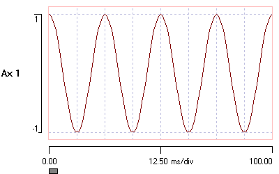
- Load the file sine 40Hz.
This shows a 40 Hz sine wave, which has been sampled at 1000 Hz. The display looks like a pretty good sine wave, but it has been highly oversampled according to the Nyquist criterion.
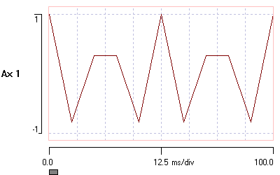
- Select the Transform: Reduce frequency menu command.
- Set the Frequency divisor to 10.
- Select the Skip intervening option (not the default Average intervening) so that you perform a true decimation.
- Click OK.


The new file does not look much like a sine wave, but since the new sampling frequency of 100 Hz is still more than twice the frequency contained within the signal (40 Hz), according to the Nyquist criterion it ought to contain all the information in the original signal.
To find out whether this is true:
- With the new file active, select the Transform: Increase frequency menu command.
- Set the Frequency multiplier to 10.
- Keep the Type as Filter.
When the operation completes, the new interpolated file will load. Note that the original sine wave has been reconstructed very accurately, although there has been a slight loss of amplitude because the process is not perfectly efficient (nothing ever is). Also note that the end part of the file has been set to 0 due to the inevitable loss of some data due to filter windowing.
If you want to be persuaded of the importance of the Nyquist criterion, then repeat the process but this time reduce the sample frequency by a factor of 20. This breaks the Nyquist rule – the resulting 50 Hz sample frequency is less than twice the frequency of the 40 Hz sine wave that is contained in the data. If you now increase the frequency by a factor of 20, you end up with a very nice-looking sine wave, but it has completely the wrong frequency, 10 Hz rather than 40 Hz! This is an example of data aliasing – a phenomenon in which data can look convincing but be completely wrong
Interpolation algorithm
The Increase frequency command works as follows. It produces (but does not display) an intermediate file consisting of the original (reduced frequency) data values, but with each real sample value interspersed by an appropriate number of 0-valued samples so as to bring the file up to a length appropriate for the new increased sample frequency. This file is then passed through a low-pass filter with a cut-off frequency set at the Nyquist frequency of the original (reduced frequency) file.
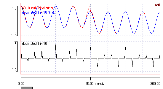
- To see this in action, load the file sine 40 decimated 10.
Like the previous file, this has a sample frequency of 1000 Hz. The top trace shows a 40 Hz sine wave, with the initial 100 ms having a slight DC offset to provide a timing reference. The lower trace shows the same data, but 9 out of every 10 samples have been replaced by a 0 value. (This was done externally to Dataview in Excel.) The peaks of the resulting positive and negative spikes are what would form the envelope of the upper-trace waveform if its sample rate had been reduced by a factor of 10. This trace is what is contained in the (hidden) intermediate file that is used when increasing the frequency by a factor of 10.
- Select the Transform: Filter: FIR filter (window sinc) menu option, and note that by default it is set to the Band pass option.
- Set the Trace to process to 2.
- Set the upper cut (Hz) to 50.
This value is appropriate because with the 10-fold sample rate reduction of trace 2, we have set its effective sample rate to 100 Hz, so 50 Hz is its Nyquist frequency. - Click the Preview button to see what the filtering will produce – hopefully it will look like a sine wave.
- Now click OK to write a new file with a new filtered trace.
When the new file loads, you should see that the 3rd (bottom) trace looks like a reduced-amplitude version of the original (top trace) sine wave. In fact, the process reduces the amplitude by the same factor as the sample-rate change, i.e. 10-fold. This is because 9 out of 10 samples in the source had amplitude 0, and this gets "shared out" amongst the non-zero values during reconstruction.
We can check this as follows:
- Selecting the Traces: Experimental gain menu command.
- Select the Traces: format menu command. In the Trace format dialog:
- Deselect Axis 3.
- Set the axis for trace 3 to 1.
- Set the colour of trace 1 to red:
click the red Colour choice button at the bottom of the dialog, then click the colour button for trace 1. - Set the colour of trace 3 to blue.
- Click OK to dismiss the dialog. The
The reconstructed sine wave (blue trace) now overlies the original sine wave (red trace) almost exactly, except at the time of the apparent step change in amplitude at 100 ms, where there is a gradual rather than abrupt transition.
