Contents
Principal component analysis
Background
PCA Schematic
Artificial data
No noise
With noise
PCA with n > p
Weird data
Clustering
Real spikes
Principal Component Analysis (PCA)
This tutorial gives a conceptual overview of principal component analysis and mainly uses artificial data. A hands-on walk-through using real data is available here.
Background
What is principal component analysis? Here is one conceptual definition:
The central idea of principal component analysis (PCA) is to reduce the dimensionality of a data set consisting of a large number of interrelated variables, while retaining as much as possible of the variation present in the data set. This is achieved by transforming to a new set of variables, the principal components (PCs), which are uncorrelated, and which are ordered so that the first few retain most of the variation present in all of the original variables. (Jolliffe, 2002).
That is fine, but how does it relate to neurophysiology?
A common use of PCA in neurophysiology is to help with spike sorting from extracellular recordings. If you use a template- or threshold-based search procedure to detect the spikes, you will end up with a series of events each of which marks a putative spike. The spike waveforms are the "interrelated variables" of the definition above, and are likely to have quite similar, but not identical, waveforms. Some of the variability is simply due to noise, but some is because the waveforms are generated by different axons. These waveforms are likely to fall into into shape clusters, each of which you would interpret as containing spikes from a different axon.
PCA is a technique that automatically "repackages" the spike waveforms into another set of waveforms called basis waveformsThey are also sometimes called the Eigenvectors, loadings vectors, coefficients or just factors. It can get confusing!. These emphasize the differences in the original set of spike waveforms, and there is no correlation between the various basis waveforms (they are orthonormal) so there is no redundant information between them. PCA also gives you a series of weighting coefficientsSometimes called scores. that tell you how much each point in each basis waveform contributes to the original spike waveform. The original spike waveforms can be recovered by summing the basis waveforms, but with each point multiplied by the appropriate weighting coefficientThe original waveform is thus a linear combination of the basis waveforms, which is why PCA is a procedure within the mathematical discipline of linear algebra..
At first sight it might seem a pointless exercise to switch waveforms from one package type to another. However, the key advantage is that the new packages (the basis waveforms) are automatically sorted in the order of information importance, where the first reflects the greatest variability in the spike waveforms, the second reflects the next greatest variability, and so on. PCA can also tell you how much information is contained in each basis waveform, often displayed as a list of EigenvaluesThe name derives from the mathematical procedure used to calculate them. which describe the amount of variance explained by the package. Because the basis waveforms are in order of information importance, you only have to use the first few (often just the first 3), to recover a close approximation to the original waveforms.
In spike sorting, PCA is not usually used to recover spike waveforms - in fact, the basis waveforms are often not used at all. For spike sorting, the important information is contained in the weighting coefficients, since it is the differences between these that turn the single set of basis waveforms into the multiple sets of spike waveforms. So these are what are clustered, rather than the original waveforms (and certainly not the basis waveforms, since these are all totally uncorrelated with each other and therefore don't form clusters). The important advantage is that instead of trying to cluster based on differences in the full waveforms of the detected spikes, much of which is due to noise, you try to cluster based on the differences between just the first few sets of weighting coefficients, very little of which is due to noise. This is much more likely to be successful, and that is why PCA is often used in spike sorting.
PCA Schematic
It is easy to got lost in the terminologyIt is not helped by the fact that different disciplines tend to use different naming conventons for the same components in PCA. of PCA and the dimensions of the data, so a schematic illustration might be helpful.
Assume that we have n spikes, each with a waveform containing p sample values. There is going to be a lot of correlation between these waveforms, because if the peak value of a spike occurs at sample x in one waveform, a similar value is likely to occur at or near sample x for all the other waveforms generated by the same axon (barring spike overlap). This of course assumes that the spike waveforms are properly aligned, but that should be built into the spike detection algorithm.
The PCA produces 3 sets of numerical output values:
- The first is the set of n uncorrelated basis waveforms, each of the same length p as the original input waveforms.
- The second is a list of n Eigenvalues which are often expressed as a percentage that specifies the amount of the variance explained by each of the n basis waveforms. Very often only the first few values are significantly greater than 0, indicating that only the first few basis waveforms contain useful information.
- The third is an n x n matrix of weighting coefficients.
The relationship between the various elements is expressed in the equation:
\begin{equation} \mathsf{R}_{x, k} =\sum _{j=1}^n \left(\mathsf{B}_{x,j} \times \mathsf{C}_{k,j}\right) \label{eq:eqPCA} \end{equation}where R is the p x n matrix of raw spike waveforms, B is the p x n matrix of basis waveforms, and C is the n x n matrix of weighting coefficients. Subscript x is the sample index (1 : p), k is the spike index (1 : n), and j is the basis waveform index (1 : n). Normally a close approximation to R can be achieved by summing from j = 1 to j = 3 or 4, rather than to the full value of n.

Artificial Data
We will look at PCA of some artificial data with a very simple structure. This has the advantage of yielding numerical results that we can actually understand!
- Load the file pca demo.
- Activate the Event analyse: Event-triggered scope view command to become familiar with the data.
- Click the Disp=Ev (1) button.
- Look at each of the 6 sweeps triggered by channel a in turn by incrementing the Hightlight sweep parameter from 1 to 6.
Note that the event waveforms in the top trace consist of a triplet series of stepped pulses, the first part in each triplet has a fixed amplitude of 12, the second part has varying amplitudes of 9, 6 and 3 in turn. The second trace is identical to the first except that it has some additional random noise. The third trace is completely flat (zero-valued), and the fourth trace is flat but with added noise. The latter two traces are just there to explore the limitations of PCA with unusual data.
Each event waveform in each channel is 10 samples long - you could check this with the Num samples option in the Event parameter list. The only difference between the event channels is that a detects the first 6 waveforms (so n < p), b detects the first 12 waveforms (so n > p) , and c detects all 108 of the waveforms (so n >> p).
- Close the Scope view.
- Select the Event analysis: Shape classification/clustering: Principal components analysis: Calculate command to show the Principal Component Analysis (Covariance) dialog.
This dialog performs PCA using an algorithm known as "Eigen-reduction of the covariance matrix". The mathematical details of this do not matterAnd I am completely incapable of explaining them - but there are plenty of maths textbooks and websites that do. for this tutorial, but it is important to realize that it becomes prohibitively slow with large data sets (> ~500 events). For analysing such data you should use the Event analysis: Shape classification/clustering: Principal components analysis: Quick calculate command. This implements a different algorithm (NIPALSnon-linear iterative partial least squares) which is much faster but does not give so much detail.
No noise
There are 6 events in the default event channel a, so potentially 6 PCs. One would normally only be interested in the first few, but for the sake of the tutorial we will look at all of them.
- Set the Number of PCs to 6.
- Click the Calculate button at the bottom left.
Note that the default trace is 1, which has no noise associated with it.
The results of PCA show as text in the edit box in the dialog. At the top is a reminder that there are 6 events, each 10 samples long. So using the previous notation, n = 6 and p = 10.
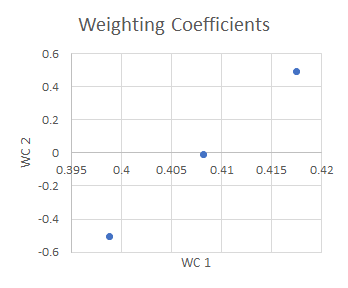
Eigenvalues: Below that are the 6 (n) Eigenvalues, but only the first 2 are non-zero. This tells us that only the first two basis waveforms contribute anything to defining the waveforms.
Weighting coefficients: Next comes the 6 x 6 (n x n) matrix of weighting coefficients. This is fully populated, but actually only the first 2 columns would be needed to reconstitute the waveforms - the other columns would end up multipling a zero-valued element in the basis waveforms.
Note that the values in the first 2 columns are identical recurring triplets, which fits with the fact that there are 3 types of identical waveforms. The values in the remaining columns are not triplets, but these have no significant associated Eigenvalues.
| #event | WC 1 | WC 2 |
| 1 | 0.4175 | 0.4923 |
| 2 | 0.4082 | -0.0076 |
| 3 | 0.3988 | -0.5075 |
| 4 | 0.4175 | 0.4923 |
| 5 | 0.4082 | -0.0076 |
| 6 | 0.3988 | -0.5075 |
Basis waveforms: Finally, there is the 6 x 10 (n x p) matrix containing the basis waveforms, but only the first 2 contain non-zero elements.
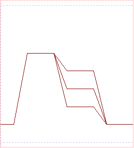
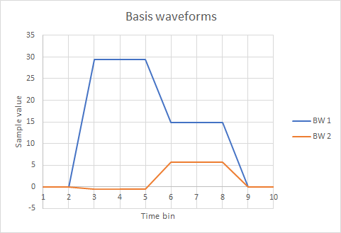
The first basis waveform (BW 1) reflects the “dominant” shape common to all the waveforms, but the second basis waveform does not look like any of the original waveforms. The second and subsequent basis waveforms act like “correction factors” that, when summed with the first basis waveform in varying proportions, reconstruct the original data. The correct proportions are determined by the weighting coefficients. Remember that there is no noise in this sample set, and that the waveforms only differ in one parameter - the size of the second step. So intuitively it makes sense that there are only 2 non-zero basis waveforms - one to define a core shape (but this is not numerically identical to the shared first part of the raw waveform), and the other to make the single parameter adjustments.
To see this in action let us reconstruct the 6th sample of the 2nd waveform using formula \eqref{eq:eqPCA} above. This element has an actual value of 6 (we could measure it in the Scope view, but I know it because it was constructed that way). Taking the data from the PCA output in the dialog, we have:
| Weighting coefficients | ||||||
| #event | WC 1 | WC 2 | WC 3 | WC 4 | WC 5 | WC 6 |
| 2 | 0.4082 | -0.0076 | 0.2624 | 0.2733 | -0.8293 | 0.0452 |
| Basis waveforms | ||||||
| time bin | BW 1 | BW 2 | BW 3 | BW 4 | BW 5 | BW 6 |
| 6 | 14.8065 | 5.7243 | 0 | 0 | 0 | 0 |
| Product WC x BW | ||||||
| 6.044013 | -0.0435 | 0 | 0 | 0 | 0 | |
If we sum the products of the WC and BW values in each column we get 6.0005, which is within rounding error of the real value. Furthermore, it is obvious that only the first two basis waveforms contribute anything because the BW multiplier is 0 for all the others.
With noise
- In the PCA dialog, set the Trace to 2.
- Click the Calculate button.
A new PCA is performed, and this time there are no zero-valued elements in the output. However, the first 2 Eigenvalues are much bigger than the rest, and account for nearly all (99.8%) of the variability in the data. This makes sense because trace 2 is identical to trace 1 except that there is added noise. The first 2 basis waveforms are needed to describe the core waveforms, the remaining just describe the noise that is different for each event, and which is thus totally uncorrelated between events.
The actual value of sample 6 of event 2 in trace 2 is 5.6273 (i.e the core value of 6 perturbed by some noise). The relevant data for reconstruction are:
| Weighting coefficients | ||||||
| #event | WC 1 | WC 2 | WC 3 | WC 4 | WC 5 | WC 6 |
| 2 | 0.4063 | 0.0097 | 0.5529 | -0.5344 | -0.4866 | 0.0821 |
| Basis waveforms | ||||||
| time bin | BW 1 | BW 2 | BW 3 | BW 4 | BW 5 | BW 6 |
| 6 | 14.858 | 5.8999 | -0.4178 | 0.0287 | 0.4393 | -0.082 |
| Product WC x BW | ||||||
| 6.0368 | 0.0572 | -0.231 | -0.0153 | -0.214 | -0.00673 | |
If we reconstruct by summing the full set of 6 WC x BW products we get 5.6272, which is very close to the original real value. However, if we sum using just the first 2 products, which are the ones with significant Eigenvalues, we get 6.0940, which is actually closer to "real" value before noise was added.
PCA with n > p
- In the PCA dialog, set the Event channel to b, the Trace to 2 and the Number of PCs to 12.
- Click Calculate.
We are now analysing 12 waveforms, each 10 samples long. The calculation produces 12 basis waveforms, but the last 3 (10, 11 and 12) are flat lines, although not zero valued. Furthermore, the Eigenvalues drop to 0 from 10 onwards, and so the associated PCs contain no useful information. This emphasizes the point that the purpose of PCA is not to reconstruct the original waveforms exactly - that would indeed be pointless, since we already have them. The purpose is dimensionality reduction, and for that we usually only need the first few PCs.
Weird data
What happens if you attempt PCA on innapropriate data?
Flat line
- In the PCA dialog, set the Trace to 3, leaving the other parameters unchanged.
- Click Calculate.
Trace 3 is completely flat, and the PCA algorithm fails to produce sensible output. The Eigenvalues are listed as "nan" (which means "not a number") and all other values are 0. This is because the algorithm works on the covariance matrix, and if all the numbers are equal, there is no variance at all.
Nothing but noise
- In the PCA dialog, set the Trace to 4.
- Click Calculate.
Trace 4 is nothing but noise. The Eigenvalues do not show a sudden drop at any level - there is just a gradual decline. In fact, with some settings (e.g. with event channel a selected), the Eigenvalues are not even in order. This is because to be a sensible procedure, PCA requires there to be some correlation between the raw waveforms. If all the waveforms are random noise and hence completely uncorrelated with each other, none of the basis waveforms is any better than any of the others at "explaining" the variability in the data, and the procedure is pointless.
Clustering
As stated at the beginning, PCA is routinely used for spike sorting by clustering the weighting coefficients. We can try this out with the artificial data, which has the advantage that we know that there are just 3 clusters (reflecting the 3 sizes of the second step in the waveforms), and we know exactly which cluster each waveform belongs to.
- If necessary, move the PCA dialog so that it does not obscure the events displayed in the main view.
- Set the event channel to c, the trace to 2, and the Number of PCs to 3.
There are 108 events in this channel. The number is somewhat arbitrary, but it is certainly the case that the more data you present for clustering, the more likely it is that the clustering algorithm will succeed (so long as clusters do actually exist). If you attempt to cluster just the 12 events in channel b, all the data are put into a single cluster.
- Click the Calculate button.
- Click the Cluster button.
- Click the Cluster button in the new Cluster dialog that displays.
The cluster algorithm should find 3 clusters, as indicated by the 3 coloured markers on the right of the display: red, cyan and blue. In the Cluster statistics of the Cluster dialog note that the proportion (prop) of each cluster is 0.333 (i.e. one third). This fits with the triplets of waveform shapes in the data. The event markers in the main display should now be coloured. Every third event (e.g. 1, 4, 7 etc.) should have the same colour, because its waveform belongs to the same member of the triplets.
- Click OK in the Cluster dialog to "lock in" the colours.
- Click the Partition button in the PCA dialog.
- Click OK to accept the defaults in the new Partition dialog that displays.
- Close the PCA dialog.
There should now be 3 new event channels (d - f) in the data file, each marking one of the event waveforms.
- Re-activate the Scope view.
- Re-activate the Scope view with the Event analyse: Event-triggered scope view command.
- Click the Disp=Ev (1) button.
- Select from Events in the Sweep Colours group (about half-way down on the left).
- Set the Trigger channel to c, d, e and f in turn to see the waveforms marked by the events in these channels, coloured according to the colours of the events in each channel
Real Spikes
A walk-through of spike sorting using PCA with real data is given here. However, that uses the quick calculate (NIPALS) algorithm and does not give access to the basis waveforms, so it is worth a quick look at real data using the covariance method.
- Load the file r3s 58.
- Set the timebase of the main view to 32 ms/div to see more of the data.
Note that spikes have already been detected as described here. - Activate the Event analyse: Event-triggered scope view command to open the Scope view dialog.
- Set the count to -1 to see all 542 spike waveforms.
There are 4 obviously distinct spike shapes.
- Set the count to -1 to see all 542 spike waveforms.
- Select the Event analysis: Shape classification/clustering: Principal components analysis: Calculate command to show the Principal Component Analysis (Covariance) dialog.
- Set the Number to calculate to -1 to use all 542 waveforms.
- Click Calculate.
After a pause the results should display. There are 42 samples in each spike waveform, but only the first 16 Eigenvalues are shown because after that the percentage variance drops below 0.001%, which is essentally 0. In fact, the first 3 Eigenvales account for 99.7% of the variance, so the first 3 basis waveforms contain nearly all the information about the spike shapes, and only the first 3 weighting coefficients would be needed for spike sorting.
For comparison, the raw spike waveforms and their first 3 basis waveforms are shown below.
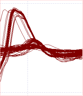
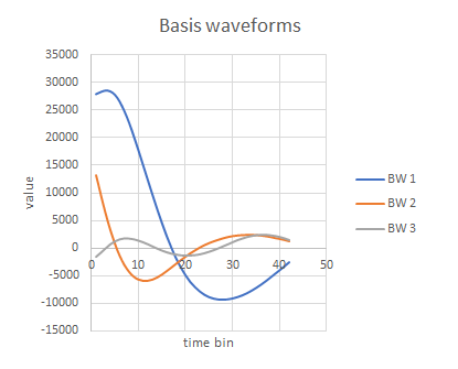
The first basis waveform looks rather like the raw waveform of the largest spike in the recording, (although it is by no means identical to it and cannot form any sort of template) and that makes sense because this waveform has the greatest variability in the sample, and so contributes most to the first basis waveform. However, the other two basis waveforms do not look anything like the raw spike waveforms. This is because, as stated previously, they act as "correction factors" to the first basis waveform, rather than as spike waveforms in their own right. Furthermore, there is no correlation between the basis waveform values at a particular sample time, whereas there is considerable correlation in the raw waveforms at any sample time - as is evidenced by the fact that many of the spike waveforms more-or-less superimpose on each other.