Event Spectrum Analysis

It is sometimes desirable to perform spectral analysis on data within events, and to ignore all other data.

• Load the file sine events.

 

There are 3 events, and trace 2 contains a single cycle of a sine wave within each eventThis was constructed using the Transform: Set data value in events command, using the equation sin((1000/ed)*2*_pi*et/1000) .. The aim is to measure the frequency of the sine wave within each event. The event durations (ms) are shown as labels for each event.

• Select the Event analyse: Frequency spectrum menu command to open the Event Spectrum Analysis dialog box.

Normally it would be advisable to set appropriate dialog entries before attempting analysis, but for the sake of instruction, we will dive straight in.

• Click the Analyse button at the bottom-left of the dialog.

By default, the spectral display shows the logarithmFor natural signals the log of the power is often more informative than the linear value of the power, because the latter tends to be dominated by the carrier frequency. of the power at various frequencies. However, there is an immediate warning that the spectrum contains 0-value power entries, and that therefore a log display is impossible and it will switch to linear. The display then shows a flat line with 0 value. This is because by default the data being analysed are in trace 1. This is a flat line with a value of 0 throughout, yielding a power of 0 at all frequencies. This can be seen in the text read-out at the top-right of the dialog. The log of 0 displays as not-a-number (-inf).

• Change the Trace to 2.
• Click Analyse.

Now at least something is visible in the display.

By default, the process will use all the events in the selected channel to calculate the spectrum. This is appropriate if differences between event data are just due to noise, but not if we want to analyse the frequency spectrum of data within each event individually. The latter is the case here.

• Set the Count (near the top of the dialog) from -1 to 1. This means that just data from the single Start at event will be analysed. (The initial value of -1 meant that all events from Start at to the last event are analysed.)
  Now, only the data within event 1 (the Start at event) are analysed.

Re-analysis occurs automatically when the Count parameter is changed, but there is no obvious change in the spectral display. This is because we do not have adequate frequency resolution to detect the change.

The Frequency resolution is set by the number of data bins passed for analysis, which by default is 64. Given the sample interval of the data (0.1 ms), this means that the frequency resolution is 78.125 Hz. The three sine wave frequencies within the data are all within this value and thus cannot be resolved. We need higher resolution.

• Click the up spin button for the Frequency resolution until it reaches 1024.

The frequency resolution is now 4.88 Hz, which might just be adequate. However, something weird happened at the last click. The spectral display trace becomes a flat line again!

This is because the 1024 frequency resolution requires 204.8 ms of data to be passed to the FFTFFT: fast Fourier transform. This is the mathematical algorithm that underlies spectal analysis. However, it only works on data segments that are a power-of-2 in length. routine for analysis (shown in the FFT dur read-out), but event 1 only contains 125 ms of data. What can be done?

To increase frequency resolution requires that more data be sent for analysis, but the amount of data available is limited by the event duration. However, if you run out of data you can simply pad the data to the required number by adding 0s. The zeros contain no power so do not affect the shape of the spectrum, although they will reduce the absolute numerical value of the power itself. But that is rarely of interest - one is usually only interested in the relative power at different frequencies.

• Check the Pad fragments box.

Now the 125 ms fragment of data in event 1 is padded with zeros to bring it up to 204.8 ms in length, and analysis can be performed.

It is now time to look at the spectrum in more detail.

• Uncheck the Autoscale X box.
• Set the right-hand X axis scale to 40.

Peak power occurs at 9.766 Hz, which is getting close to the correct value of 8 Hz. Can we increase the resolution further?

• Click the up spin button for the Frequency resolution until it reaches 16384.

The dialog should now look like this:

 

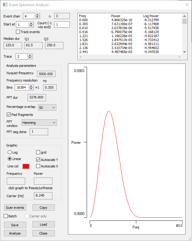
The resolution is now 0.305 Hz, which should be fine for distinguishing the 3 different frequencies in the events.

• Hover the mouse over the peak in the spectral display, and note that Frequency read-out is about 8 Hz. This is indeed the frequency of a sine wave with a cycle period of 125 ms.
• Set the Start at value to 2, to analyze data in the second event.
  Note that the peak in the spectrum display shifts to the right, and if you hover the mouse over it, the frequency read-out is now about 16 Hz.
• Finally, set the Start at value to 3, to analyze data in the third event.
  The peak in the display shifts to the left, and occurs at about 4 Hz.

Note that although the peaks of the spectrum display are in the right location, the peaks is quite broad. In principle, this implies that the data contains a range of frequencies on either side of the peak. However, in practice it can also represent uncertainty in the analysis, which is the case here. The FFT routine at this resolution requires 16385 samples, but only a relatively small fraction of these contain any useful information - the rest are zero padding. The peaks would be narrower if the events were longer and contained more cycles of the sine wave, and hence less padding. This is born out by the fact that the width of the peak depends on the duration of the event: the narrowest peak is associated with event 3, which has more data samples within it than the others.

Carrier Frequency

The frequency with the highest power level in a spectrum is known as the carrier frequency. You can find the carrier frequency for each event using the Scan events facility. The frequency is stored within the variable value associated with the event.

• Click the Scan events button.
• Call up the Event channel properties dialog box from the Event edit: Event channel properties menu command.
• Select Carrier frequency from the Numeric display per event drop-down list.
• Click OK (or Apply) in the Properties dialog box.

Note that the labels for each event now show the carrier frequency of data within the event (previously they showed the event duration). Note that the carrier frequency is calculated by spectral analysis, it is not simply the reciprocal of the event duration, although this yields a similar numerical value.

The carrier frequency is now stored with each event, and can be retrieved and listed or graphed through the various event analysis options (graph, histogram, list etc).

See also ...

For an example of event spectral analysis applied to real data (fly courtship song), see here.

 

---