Fluorescent (calcium) image pre-processing

DataView is primarily intended for analysing electrophysiological data, but it has some facilities that may be useful for fluorescent image analysis when fluorescence intensity is recorded as a series of values at equal-spaced time intervals. For example, in calcium imaging experiments, a transient increase in fluorescence in a localized patch of tissue indicates a brief increase in the concentration of free calcium within that patch, which in turn might indicate an increase in synaptic and/or spiking activity in that region.

DataView does not have any facility to interact with a camera directly. The assumption is that image capture is done externally and that the data are then exported in a format that DataView can read. This might typically be a CSV file, wih each column containing the time series from a separate region of interest. The columns are then imported as separate traces in DataView.

Photo-bleach compensation

In a calcium imaging experiment, the amount of fluorescence depends on the calcium concentration, but it also depends on the amount of the calcium-sensitive fluorophore present. One common problem is that when a fluorophore is exposed to light at its excitation frequency, it can be gradually but irreversibly destroyed in a process is known as photo-bleaching. This means that the emission of fluorescent light decays over time, and this can contaminate any signals due to variations in calcium concentration.

The precise molecular mechanism of photo-bleaching is not entirely clear, but empirical studies show that it often follows a negative mono- or bi-exponential time course, with a decline to some steady-state value representing the intrinsic tissue fluorescence plus that emitted by any unbleachable fluorophore.  The background fluorescent can thus often be fitted to one of the following equations:

\[V_t = V_{\infty} + (V_0 - V_{\infty} )e^{-t/\tau_m} \qquad\textsf{mono-exponential}\]

\[V_t = V_{\infty} + w_0(V_0 - V_{\infty} )e^{-t/\tau_{\,0}} + w_1(V_0 - V_{\infty} )e^{-t/\tau_{\,1}} \qquad\textsf{bi-exponential}\]

where V₀ is the fluorescence value at the start of exposure, V_t is the value at time t from the start, V_∞ is the value after the exponential decline stabilises, τ_0,1 is the exponential time constant (of the 1st and 2nd exponents for bi-exponential decline), and w_0,1 is the weighting of 1st and 2nd exponents for bi-exponential decline.

The mono-exponential equation has 3 free parameters, V₀ , V_∞ , and τ₀ . The bi-exponential equation has an 2 additional free parameters, τ₁ and w₀ (w₁ is fixed as 1 - w₀).

If the raw data have a reasonable fit to one of these functions they can be transformed to compensate for the exponential decline. This is usually done by dividing the raw values by the fitted exponential values on a point-by-point basis. If the data were an exact fit to the curve, this would make the trace have a value of 1 throughout its length. The absolute numerical value of fluorescence intensity can be restored simply by multiplying all corrected values by the first uncorrected intensity level (i.e. the level before any photo-bleaching has occurred). Deviations from the fitted curve caused by transient changes in calcium concentration then become apparent as deviations from this value.

This is a proportional compensation method. An alternative linear method is to just subtract the fitted curve from the raw data (making all values 0 for a perfect fit), and then to add back the initial value.

One consequence of proportional compensation is that a deviation from the baseline that occurs early in the raw recording, before much photo-bleaching has occurred, will end up as a smaller signal in the compensated record than a deviation of the same absolute raw size that occurs late in the recording, after substantial photo-bleaching. However, this is often what is wanted, since the later signal represents a greater fractional change from baseline (and hence presumably a bigger calcium signal) than the earlier signal. A downside of proportional compensation is that any non-fluorescent noise in the signal is also amplified more in the later part of the recording than the earlier.

A major problem with either method is that genuine calcium-related signals may be included in the data from which the fit is derived, and thus the fit equation may not be a true representation of baseline photo-bleaching. This means that quantitative values derived after such photo-bleach compensation should be treated with considerable caution.

Remove Exponential Drop

Constructed data

When learning how to use an analysis technique, it is often helpful to start with "fake" data that has been constructed with known properties. That way, one can assess how well a process performs at retrieving those properties because you actually know their correct values.

• Load the file constructed exponential drop.

Two traces have been constructed; trace 1 has a mono-exponential decline, trace 2 has a bi-exponential decline, and both traces have added random noise. The equations used to construct the traces are visible as trace labels. To add to the fun, an experimental "result" has been added in the form of a square perturbation in the traces which occurs after the exponential decline has stabilized.

• Select the menu command Transform: Remove exponential drop to open the Estimate and Remove Exponential Drop dialog. (This is similar but not identical to that used to estimate a membrane time constant.)

Single exponential data

The program makes an initial estimate of the parameters of a mono-exponential decline, and the display at the top-right of the dialog shows the raw signal with the exponential curve shown as a red line superimposed on the data (for an explanation of parts of the dialog box not mentioned in this tutorial, press F1 to see the on-line help). The line is a reasonable, but not exceptionally good, fit to the data.

• Click the Preview button in the Transform group near the bottom of the dialog.

A new window opens showing the raw data in the upper trace, and the transformed data, with exponential compensation as described above, in the lower. The compensation is applied using the estimated parameters of the mono-exponential. The initial steep decline of the raw data (upper preview trace, black) is replaced by a shallow rise in the transformed data (lower preview trace, red).

• Change the value of tau 0 in the main dialog to 50, and note how much worse the fit gets, and how non-linear the Preview compensated data now are.
• Click the Guess button in the Fit group to restore the original value of 98.

The Guess method automatically estimates "reasonable" initial values for a mono-exponential decline. The initial value (V₀) is set as the first value in the recording. The fully-bleached value (V_∞) is set as the value at the Fit end time. This is initially set at a time 90% through the recording, but it can be edited by the user. Also, the value can be set as an average over a specified time before the end time to reduce noise perturbation. The Fit end time is visualized as a short blue vertical line drawn across the data towards the right-hand end of the upper graph. The initial time constant (τ₀) is set as the time at which the value has declined by 63% of the difference between the initial and fully-bleached values.

• Click the Curve fit button. The program performs iterative least-squares fitting to find the parameters that minimize deviation between the data and the mono-exponential. After a while the red curve stabilizes as new values of the 3 free parameters are calculated.
  Note: The curve fitting algorithm involves some random perturbations, so it does not always generate exactly the same result even if applied to the same data. So your values may not be identical to those I report here, but they should be close.

The fit is not very good! In particular, the fully-bleached value (V_∞) is too high. The problem is that the curve fitting routine uses data from the start of the recording up to the specified Fit end time, and this includes the experimental perturbation (the square deviation in the data trace).

• Set the Fit end time to 770, to move the time to before the experimental perturbation (note the change in location of the vertical blue line), but still in a region where the data are fully bleached.
• Set the avg end time to 50. There is now a short horizontal blue line drawn forwards from the Fit end time vertical marker. This indicates the region that the Guess routine will average to generate the initial estimate of the fully-bleached value (V_∞).
• Click Guess again. This is not strictly necessary with these data, but it does no harm.
• Click the Curve fit button again

The fit is now much better. The fitted parameter values for V₀ , V_∞ , and τ₀ are 99.9, 49.9 and 101.4 respectively, which are very close to the "correct" values of 100, 50 and 100 (from the equation used in construction). The difference can easily be accounted for by the added noise. Furthermore, and most importantly, the Preview shows that the transformed trace has entirely lost the exponential drop present in the raw data.

• Select the Linear option in the Transform group, and note that the square experimental perturbation is reduced in size, and that the noise is approximately equal across the length of the record.
• Re-select the Proportional option, and note that noise amplitude gradually increases throughout the recording, and the experimental perturbation is larger.

The different transform methods are described in detail above. Both methods are reported in the literature, and it is a matter of scientific judgement to decide which is appropriate for your data.

• Note the BIC value, which is 0.
• Select Double exponential in the Model group.
• Click Curve fit.

A new fit is generated, and the red line in the upper graph looks like as good a fit as previously, and the transformed Preview also looks very good. The fitted parameters V₀ , V_∞ , and τ₀ have almost identical values to the single exponential fit. However, the Iterations done value is 100, which is the set maximum, indicating that the convergence criterion was not actually met within 100 iterations of the fit algorithm (confirmed by the fact that the delta value is 0.1 %, which is considerably above the 0.01% threshold). There are now 3 options: click Curve fit again, and see if convergence can be achieved with more iterations (possibly increasing the Maximum iterations value); reduce the Step size and then click Curve fit again, to see if more fine-grained alterations in parameters achieve convergence; or, finally, just accept that the bi-exponential model is not as good as the mono-exponential model.

• Click Curve fit again.

The fit reaches convergence after a further 60 iterations. However, the new τ₁ value is very small, and it has a very low weighting (0.03), so it makes almost no contribution to the shape of the curve. The BIC value is 11, which is larger than for the mono-exponential model. On this basis, we should reject the double exponential model in favour of the single exponential, and we did not need to worry about the lack of convergence in the former.

Double exponential data

• Change the Trace ID to 2.
• This analyses the trace that was constructed as a bi-exponential.
• Click Guess.
• Note that this switches the Model to Single exponential, and generates initial estimates for a curve of this type. The initial fit is obviously not very good.
• Click Curve fit.

The generated fit reaches convergence, but while it is not appalling, but it is not very good either. In the Preview, there is an obvious deviation from a flat line in the early part of the trace.

• Note the BIC value, which is >500.
• Select Double exponential in the Model group.
• Click Curve fit again.

The fit is now much better (the red line closely follows the data in the upper graph), and the Preview now shows a reasonably flat line in its early part. The fitted parameters V₀ , V_∞ , and τ₀ have almost identical values to the single exponential fit, but the new τ₁ value is 21.1, and it has approximately equal weighting with τ₀. This is what would be expected from the equation that generated the raw data. Furthermore, the BIC value is now just 8, which is substantially lower than that for the single exponential fit, indicating that improved fit quality is worth the added complexity of fitting 5 parameters rather than just 3.

The steps to save a single transformed trace are described below.

• Now Close the dialog.

Real data

Working with constructed data is a useful proof of principle and learning method for an analysis technique, but what really matters is how it performs with real data, which may not completely obey the theoretical rules.

• Load the file real exponential drop.

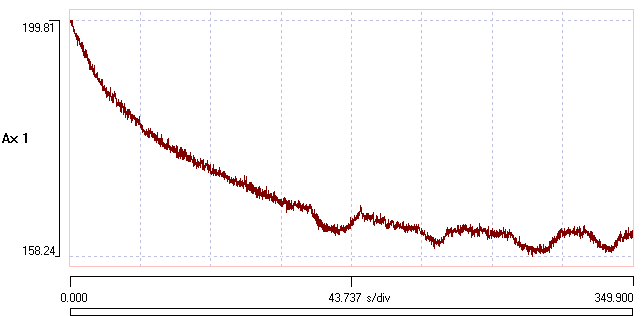
This contains 8 traces representing calcium fluorescence levels recorded at 8 different regions of interest in a fly larva that has been genetically engineered to express a calcium-sensitive fluorophore. There is a very obvious exponential-like decline in the signal level over the period of the recording in each trace.

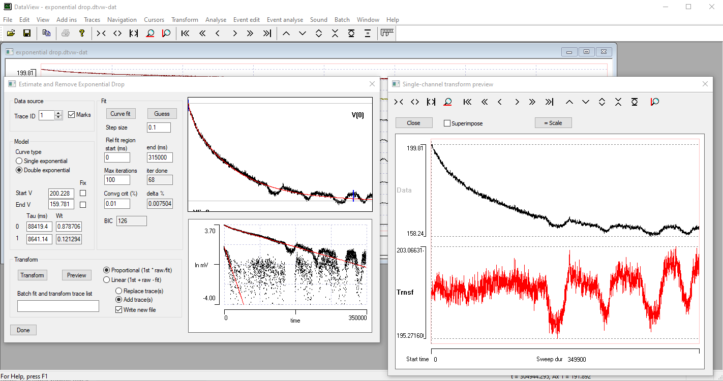
• Select the menu command Transform: Remove exponential drop to re-open the Estimate and Remove Exponential Drop dialog.

As before, the program makes an initial estimate of the parameters of a mono-exponential decline, and the display at the top-right of the dialog shows the raw signal with the exponential curve shown as a red line superimposed on the data. The line is a reasonable, but not exceptionally good, fit to the data. The BIC value is 1823.

• Click the Preview button in the Transform group near the bottom of the dialog.
• Click the Curve fit button.

The BIC value is now 460, confirming that the fitted curve is a better fit than the initial estimate. However, the fitted line clearly deviates from the raw data in the early part of the record, as shown by both the upper main graph and the Preview transform.

• Select Double exponential in the Model group.
• Click Curve fit again.

When the curve stabilizes, note that the BIC value has dropped to 126, indicating that the improvement in the fit brought about by fitting the double exponentials is “worth it” compared to the mono-exponential, even though it requires more parameters. The transformed data are now reasonably linear when viewed in the Preview window.

What Could Possibly Go Wrong?

The fit process stops when either the convergence criterion is met, which means that the percentage change in parameters values is less than the specified criterion for 3 successive iterations, or when the number of iterations reaches the set Maximum iterations. In the latter case, you can run the fit again to see whether the criterion can be reached with further iterations, or just work with the parameter values that have been achieved so far.

If the data are a poor fit to the model, the fit parameters may go off to extreme and obviously incorrect values. This is flagged by a message saying the fit “Failed to converge”, followed by restoration of the original parameters. You could try reducing the iteration Step size to see whether that helps, or manually adjusting the starting conditions to try to get a better initial fit. But if the data are too distorted, automatic fitting may be impossible, and you have to abandon the transformation, or accept the best fit that you can achieve by manual adjustment.

Manual Transform a Single Trace

At this stage, you could save the individual compensated trace to a file simply by clicking the Transform button. Before doing this you should select whether to write a new file or overwrite the original (only possible for native DataView files), and whether to add the transformed trace as a new trace, or to replace the existing raw trace.

Auto-Transform Multiple Traces

There are 8 traces in the exponential drop file, and it would be tedious to manually transform each in turn. However, we can batch process traces so that the steps are carried out automatically

• Enter 1-8 into the Batch fit and transform trace edit box in the Data source group at the top left of the dialog.
• Ensure that the Write new file box is checked (it is by default).
• Select the Replace trace option.
• Click the Transform button.
• Watch the Progress dialog box as each trace is processed (described below). You can click Cancel to stop the process, or Skip if you want to ignore a trace.
• Enter a new file name when prompted, followed by a comment if desired.

Auto transform process

The auto transform process first sets the Maximum iterations to 1000 to give some spare capacity. It then takes each selected trace in turn. It first calls the Guess routine to get initial parameters in the right range (hopefully), and then tries to fit first a mono- and then a bi-exponential curve to that trace. If there is a failure to converge, the step size is reduced from the user-specified value (to a minimum of 0.01) and the fit is retried. Whichever fit has the lower BIC value is used to transform the trace. The Progress box (below) shows which traces have been processed, the BIC values and number of iterations for each fit attempt, and the exponential type finally used in the transform. During fitting, the Progress box allows you to Skip a trace (if fitting is obviously not working) or to Cancel the whole process.

• When all traces have been processed, the Progress box exposes a Close button (and hides the Skip and Cancel buttons).

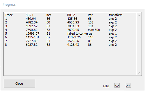
The Progress dialog above shows that the bi-exponential fit for trace 4 did not converge within the Maximum iterations (1000), but that its BIC was still (just) below that for the mono-exponential and so has been used. The bi-exponential fit for trace 5 shows the “failed to converge” message, and so the mono-exponential fit, which converged successfully, has been used. [Note that you cannot compare BIC values between traces – they are only useful for comparing fits of different models to the same data.]

• Click Close to dismiss the Transform dialogs. The new file with transformed traces loads automatically.

Adjusting the display

When the new file loads, the traces all auto-scale so that all the data are visible in each axis. However, this can obscure differences in the amplitude excursion of the various traces, which may be a key feature of the calcium image.

• Click the Same scale button () in the main toolbar (also available as the Traces: Same scale menu command).

This sets all the axes to have the same scale as axis 1. However, the different traces have different fluorescent baselines, so many are displaced outside their axis limits.

There are two possible solutions to visualize the data more comprehensibly. One is to shift the traces individually up or down until each lies within its axis limits, without changing their scale. This is a purely cosmetic change that does not affect the data. The other is to apply an offset to the actual data of each trace, so that they all have the same baseline value. This changes the data themselves, and should ONLY be done if the baseline value is irrelevant, perhaps because you are only interested in changes from the baseline (and it should be properly documented in any report).

We can try each in turn.

• Press the "v" key to add a vertical cursor, and drag it fully to the left so that it is located at time 0.
• (You could have set this explicitly using the Cursors: Place at time menu command.)
• Select the Transform: Align trace baselines menu command to open the Align Trace Baselines dialog box.
  • Select Shift scales as the Align method at the top of the dialog.
  • Leave the Master trace ID at 1.
  • Enter 2-8 in the Traces to align edit box.
  • Click OK.

The axis scales of traces 2-8 have been adjusted so that the start of each trace now lies within its axis limits at the same relative position as trace 1, and all traces are at the same scale. However, many traces overlap each other and are hard to distinguish.

• Hold down the control key, and click the gain down toolbar button () twice.
• The display now looks better.
• Select the View: Matrix view menu command to open the Trace Matrix View.
• It displays with a 3 x 3 row column matrix, because that was pre-set in the source file. You could change this if you wished by clicking the Configure button.

Some traces still go outside their axes limits, and there is "dead space" below each trace, so some adjustment is needed.

• Click the Sel all button in the Matrix view.
• You could avoid this step by holding down the control key for the subsequent steps.
• Click the Gain down toolbar button ().
• Click the down trace button () in the main toolbar.

The Matrix view now shows each trace positioned within its own axis. The traces are at the same gain, so amplitude comparisons can be made visually, but absolute DC level of each trace is different: they have been vertically-shifted to bring them into view.

A final method to visualize the data that might be useful is the Cycle traces view.

• Select the View: Cycle trace view menu command to open the Cycle Trace View.

The Cycle trace view displays all the traces on the same axis, so now the real difference in baseline means that some traces are out of view. It is time to try the other adjustment.

• Select the Transform: Align trace baselines menu command to again to re-open the Align Trace Baselines dialog box.
• There should still be a vertical cursor at the left-hand end of the main view.
• Leave the Align method as the default Shift data (transform) selection.
• Leave the Master trace ID at 1.
• Enter 2-8 in the Traces to align edit box.
• Click OK.
• Leave Write new file box checked for safety - if you are confident in the procedure you could un-check it.
• Enter a new file name when requested.

When the new file loads the Cycle Traces and Matrix views automatically switch to use it as the source for data. The Cycle traces view looks good, but some traces are off scale in the Matrix view. This is because the main view has retained its previous axis scale settings.

• Click the Same scale button () in the main toolbar to bring all traces into their cells in the Matrix view.
• In the Cycle Trace View, click the up spin button control of the Selected trace edit box to view each trace in turn in the context of all the other traces.

Hopefully, between them, these 3 visualizations of the data give you enough information to decide what, if any, further analysis would be useful. The final version of the file is available here: real exponential drop transformed, so you can try the different views without going through the analysis steps yourself.

ΔF/F₀

When comparing time-series changes in fluorescence between different tissues and different experiments, it is usual to normalize the levels in some way because unavoidable differences in fluorophore loading and tissue characteristics can significantly affect absolute fluorescence levels.

One fairly standard procedure in fluorescent image analysis is to use the signal-to-baseline ratio (SBR), also called ∆F/F₀ normalization. In this, F₀ is a measure of the baseline fluorescence in the resting state, and ∆F is the moment-by-moment deviation from that baseline. Thus:

\[SBR_t = \frac{\Delta{F_t}}{F_0} = \frac{F_t-F_0}{F_0}\]

There are several different methods for determining F₀ described in the literature, and some of these are available in DataView.

• Select the Transform: Normalize: delta F/F0 menu command, which activates the Normalize dialog box with the delta F/F0 option selected.

The Camera baseline is normally left at 0, but can be set to a positive value if the imaging camera has a non-zero output even in darkness. This value is subtracted from both F_t and F₀ during normalization (unless the F₀ value is set explicitly by the user - see below).

The F0 offset is also normally left at 0, but can be set to a positive value and added to the divisor during normalization if there is a risk that on-the-fly F₀ calculation might yield values very close to zero.

There are five options for obtaining F₀ values in DataView.

1. F₀ is set to the average F_t value measured from the trace over the whole recording. This may be appropriate in a preparation that is continuously active and it is not possible to measure a "resting" value. This can yield negative ∆F/F₀ values.
2. F₀ is set to the average F_t value measured from the trace over a user-specified time window in the recording. This may be appropriate if a preparation is initially quiescent, and then something is done to activate it. The F₀ measurement can be made during the quiescent period.
3. F₀ is set to an explicit value chosen by the user. This could be useful if one of the traces contained a recording from a non-reactive region of tissue. The average value of this trace could be obtained from the Analyse: Measure data: Whole-trace statistics menu command and used directly as F₀ for the other traces.
4. The percentile filter option continuously updates F₀ throughout the recording. It does this by passing a sliding window of user-specified duration over the data, and setting F₀ to the specified percentile value (typically 20%) within the window (e.g. Mu et al., 2019). This not only normalizes F_t, but also filters the ∆F/F₀ values to emphasize transient changes at the expense of plateaus. However, it should be used with care because this filter type is not well characterized from a theoretical signal-processing perspective.
5. The lowest sum process finds the user-specified window of data in the trace with the lowest average value in the recording, and uses this as F₀. This may be useful if quiescent periods of data occur at unpredicatable times within a recording.

Note that in all these cases except the user-specified value, the F₀ value is calculated independently for each trace and applied to that trace only. If you wish to apply the F₀ value derived from one trace to all the traces in a recording, you should calculate it separately using the various analysis procedures in DataView, and then set F₀ to this user-specified value.

 

---